Repository of Reproducible Computations

Free Statistics

of Irreproducible Research!

Author's title

Author

*The author of this computation has been verified*

R Software Module

rwasp_autocorrelation.wasp

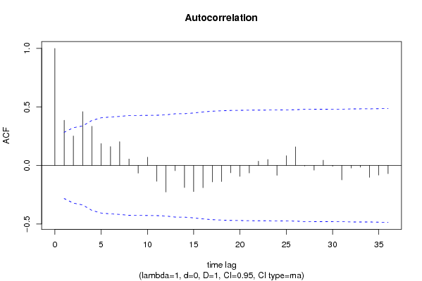
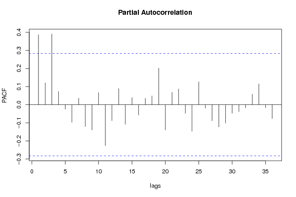
Title produced by software

(Partial) Autocorrelation Function

Date of computation

Thu, 26 Nov 2009 13:37:24 -0700

Cite this page as follows

Statistical Computations at FreeStatistics.org, Office for Research Development and Education, URL https://freestatistics.org/blog/index.php?v=date/2009/Nov/26/t12592679345z929c1dlid8k61.htm/, Retrieved Sun, 28 Apr 2024 19:46:04 +0000

Statistical Computations at FreeStatistics.org, Office for Research Development and Education, URL https://freestatistics.org/blog/index.php?pk=60386, Retrieved Sun, 28 Apr 2024 19:46:04 +0000

QR Codes:

Paste this QR Code to cite your computation.

Original text written by user:

IsPrivate?

No (this computation is public)

User-defined keywords

Estimated Impact

115

Family? (F = Feedback message, R = changed R code, M = changed R Module, P = changed Parameters, D = changed Data)

-     [Univariate Explorative Data Analysis] [Run Sequence gebo...] [2008-12-12 13:32:37] [76963dc1903f0f612b6153510a3818cf]
- R  D  [Univariate Explorative Data Analysis] [Run Sequence gebo...] [2008-12-17 12:14:40] [76963dc1903f0f612b6153510a3818cf]
-         [Univariate Explorative Data Analysis] [Run Sequence Plot...] [2008-12-22 18:19:51] [1ce0d16c8f4225c977b42c8fa93bc163]
- RMP       [(Partial) Autocorrelation Function] [Identifying Integ...] [2009-11-22 12:16:10] [b98453cac15ba1066b407e146608df68]
-    D        [(Partial) Autocorrelation Function] [WS8] [2009-11-24 18:55:10] [b8b64ced21f32e31669b267b64eede7f]
-   P             [(Partial) Autocorrelation Function] [WS8] [2009-11-26 20:37:24] [9a1fef436e1d399a5ecd6808bfbd8489] [Current]

Feedback Forum

Post a new message

Dataseries X:

Download CSV

Histogram

Boxplots

Summary of computational transaction
Raw Input	view raw input (R code)
Raw Output	view raw output of R engine
Computing time	1 seconds
R Server	'Gwilym Jenkins' @ 72.249.127.135

\begin{tabular}{lllllllll}
\hline
Summary of computational transaction \tabularnewline
Raw Input & view raw input (R code)  \tabularnewline
Raw Output & view raw output of R engine  \tabularnewline
Computing time & 1 seconds \tabularnewline
R Server & 'Gwilym Jenkins' @ 72.249.127.135 \tabularnewline
\hline
\end{tabular}
%Source: https://freestatistics.org/blog/index.php?pk=60386&T=0

[TABLE]
[ROW][C]Summary of computational transaction[/C][/ROW]
[ROW][C]Raw Input[/C][C]view raw input (R code) [/C][/ROW]
[ROW][C]Raw Output[/C][C]view raw output of R engine [/C][/ROW]
[ROW][C]Computing time[/C][C]1 seconds[/C][/ROW]
[ROW][C]R Server[/C][C]'Gwilym Jenkins' @ 72.249.127.135[/C][/ROW]
[/TABLE]
Source: https://freestatistics.org/blog/index.php?pk=60386&T=0

Globally Unique Identifier (entire table): ba.freestatistics.org/blog/index.php?pk=60386&T=0

As an alternative you can also use a QR Code:

The GUIDs for individual cells are displayed in the table below:

Summary of computational transaction
Raw Input	view raw input (R code)
Raw Output	view raw output of R engine
Computing time	1 seconds
R Server	'Gwilym Jenkins' @ 72.249.127.135

Autocorrelation Function
Time lag k	ACF(k)	T-STAT	P-value
1	0.386241	2.676	0.005082
2	0.251845	1.7448	0.043707
3	0.459798	3.1856	0.00127
4	0.334124	2.3149	0.012471
5	0.186833	1.2944	0.100857
6	0.160579	1.1125	0.135727
7	0.203151	1.4075	0.082865
8	0.055133	0.382	0.352083
9	-0.065979	-0.4571	0.324824
10	0.070507	0.4885	0.313715
11	-0.135374	-0.9379	0.176497
12	-0.227135	-1.5736	0.06107
13	-0.044469	-0.3081	0.379674
14	-0.189101	-1.3101	0.098193
15	-0.223085	-1.5456	0.064387
16	-0.190423	-1.3193	0.096665
17	-0.140681	-0.9747	0.167306
18	-0.137804	-0.9547	0.172249
19	-0.062809	-0.4352	0.3327
20	-0.09322	-0.6459	0.260726
21	-0.06395	-0.4431	0.329858
22	0.036027	0.2496	0.401979
23	0.050892	0.3526	0.362969
24	-0.084728	-0.587	0.279972
25	0.082874	0.5742	0.284268
26	0.158763	1.0999	0.138421
27	-0.004825	-0.0334	0.486736
28	-0.040117	-0.2779	0.391127
29	0.044376	0.3074	0.379918
30	-0.007269	-0.0504	0.480023
31	-0.123448	-0.8553	0.198325
32	-0.022198	-0.1538	0.43921
33	-0.015045	-0.1042	0.458707
34	-0.101795	-0.7053	0.24203
35	-0.082044	-0.5684	0.2862
36	-0.069945	-0.4846	0.315085

\begin{tabular}{lllllllll}
\hline
Autocorrelation Function \tabularnewline
Time lag k & ACF(k) & T-STAT & P-value \tabularnewline
1 & 0.386241 & 2.676 & 0.005082 \tabularnewline
2 & 0.251845 & 1.7448 & 0.043707 \tabularnewline
3 & 0.459798 & 3.1856 & 0.00127 \tabularnewline
4 & 0.334124 & 2.3149 & 0.012471 \tabularnewline
5 & 0.186833 & 1.2944 & 0.100857 \tabularnewline
6 & 0.160579 & 1.1125 & 0.135727 \tabularnewline
7 & 0.203151 & 1.4075 & 0.082865 \tabularnewline
8 & 0.055133 & 0.382 & 0.352083 \tabularnewline
9 & -0.065979 & -0.4571 & 0.324824 \tabularnewline
10 & 0.070507 & 0.4885 & 0.313715 \tabularnewline
11 & -0.135374 & -0.9379 & 0.176497 \tabularnewline
12 & -0.227135 & -1.5736 & 0.06107 \tabularnewline
13 & -0.044469 & -0.3081 & 0.379674 \tabularnewline
14 & -0.189101 & -1.3101 & 0.098193 \tabularnewline
15 & -0.223085 & -1.5456 & 0.064387 \tabularnewline
16 & -0.190423 & -1.3193 & 0.096665 \tabularnewline
17 & -0.140681 & -0.9747 & 0.167306 \tabularnewline
18 & -0.137804 & -0.9547 & 0.172249 \tabularnewline
19 & -0.062809 & -0.4352 & 0.3327 \tabularnewline
20 & -0.09322 & -0.6459 & 0.260726 \tabularnewline
21 & -0.06395 & -0.4431 & 0.329858 \tabularnewline
22 & 0.036027 & 0.2496 & 0.401979 \tabularnewline
23 & 0.050892 & 0.3526 & 0.362969 \tabularnewline
24 & -0.084728 & -0.587 & 0.279972 \tabularnewline
25 & 0.082874 & 0.5742 & 0.284268 \tabularnewline
26 & 0.158763 & 1.0999 & 0.138421 \tabularnewline
27 & -0.004825 & -0.0334 & 0.486736 \tabularnewline
28 & -0.040117 & -0.2779 & 0.391127 \tabularnewline
29 & 0.044376 & 0.3074 & 0.379918 \tabularnewline
30 & -0.007269 & -0.0504 & 0.480023 \tabularnewline
31 & -0.123448 & -0.8553 & 0.198325 \tabularnewline
32 & -0.022198 & -0.1538 & 0.43921 \tabularnewline
33 & -0.015045 & -0.1042 & 0.458707 \tabularnewline
34 & -0.101795 & -0.7053 & 0.24203 \tabularnewline
35 & -0.082044 & -0.5684 & 0.2862 \tabularnewline
36 & -0.069945 & -0.4846 & 0.315085 \tabularnewline
\hline
\end{tabular}
%Source: https://freestatistics.org/blog/index.php?pk=60386&T=1

[TABLE]
[ROW][C]Autocorrelation Function[/C][/ROW]
[ROW][C]Time lag k[/C][C]ACF(k)[/C][C]T-STAT[/C][C]P-value[/C][/ROW]
[ROW][C]1[/C][C]0.386241[/C][C]2.676[/C][C]0.005082[/C][/ROW]
[ROW][C]2[/C][C]0.251845[/C][C]1.7448[/C][C]0.043707[/C][/ROW]
[ROW][C]3[/C][C]0.459798[/C][C]3.1856[/C][C]0.00127[/C][/ROW]
[ROW][C]4[/C][C]0.334124[/C][C]2.3149[/C][C]0.012471[/C][/ROW]
[ROW][C]5[/C][C]0.186833[/C][C]1.2944[/C][C]0.100857[/C][/ROW]
[ROW][C]6[/C][C]0.160579[/C][C]1.1125[/C][C]0.135727[/C][/ROW]
[ROW][C]7[/C][C]0.203151[/C][C]1.4075[/C][C]0.082865[/C][/ROW]
[ROW][C]8[/C][C]0.055133[/C][C]0.382[/C][C]0.352083[/C][/ROW]
[ROW][C]9[/C][C]-0.065979[/C][C]-0.4571[/C][C]0.324824[/C][/ROW]
[ROW][C]10[/C][C]0.070507[/C][C]0.4885[/C][C]0.313715[/C][/ROW]
[ROW][C]11[/C][C]-0.135374[/C][C]-0.9379[/C][C]0.176497[/C][/ROW]
[ROW][C]12[/C][C]-0.227135[/C][C]-1.5736[/C][C]0.06107[/C][/ROW]
[ROW][C]13[/C][C]-0.044469[/C][C]-0.3081[/C][C]0.379674[/C][/ROW]
[ROW][C]14[/C][C]-0.189101[/C][C]-1.3101[/C][C]0.098193[/C][/ROW]
[ROW][C]15[/C][C]-0.223085[/C][C]-1.5456[/C][C]0.064387[/C][/ROW]
[ROW][C]16[/C][C]-0.190423[/C][C]-1.3193[/C][C]0.096665[/C][/ROW]
[ROW][C]17[/C][C]-0.140681[/C][C]-0.9747[/C][C]0.167306[/C][/ROW]
[ROW][C]18[/C][C]-0.137804[/C][C]-0.9547[/C][C]0.172249[/C][/ROW]
[ROW][C]19[/C][C]-0.062809[/C][C]-0.4352[/C][C]0.3327[/C][/ROW]
[ROW][C]20[/C][C]-0.09322[/C][C]-0.6459[/C][C]0.260726[/C][/ROW]
[ROW][C]21[/C][C]-0.06395[/C][C]-0.4431[/C][C]0.329858[/C][/ROW]
[ROW][C]22[/C][C]0.036027[/C][C]0.2496[/C][C]0.401979[/C][/ROW]
[ROW][C]23[/C][C]0.050892[/C][C]0.3526[/C][C]0.362969[/C][/ROW]
[ROW][C]24[/C][C]-0.084728[/C][C]-0.587[/C][C]0.279972[/C][/ROW]
[ROW][C]25[/C][C]0.082874[/C][C]0.5742[/C][C]0.284268[/C][/ROW]
[ROW][C]26[/C][C]0.158763[/C][C]1.0999[/C][C]0.138421[/C][/ROW]
[ROW][C]27[/C][C]-0.004825[/C][C]-0.0334[/C][C]0.486736[/C][/ROW]
[ROW][C]28[/C][C]-0.040117[/C][C]-0.2779[/C][C]0.391127[/C][/ROW]
[ROW][C]29[/C][C]0.044376[/C][C]0.3074[/C][C]0.379918[/C][/ROW]
[ROW][C]30[/C][C]-0.007269[/C][C]-0.0504[/C][C]0.480023[/C][/ROW]
[ROW][C]31[/C][C]-0.123448[/C][C]-0.8553[/C][C]0.198325[/C][/ROW]
[ROW][C]32[/C][C]-0.022198[/C][C]-0.1538[/C][C]0.43921[/C][/ROW]
[ROW][C]33[/C][C]-0.015045[/C][C]-0.1042[/C][C]0.458707[/C][/ROW]
[ROW][C]34[/C][C]-0.101795[/C][C]-0.7053[/C][C]0.24203[/C][/ROW]
[ROW][C]35[/C][C]-0.082044[/C][C]-0.5684[/C][C]0.2862[/C][/ROW]
[ROW][C]36[/C][C]-0.069945[/C][C]-0.4846[/C][C]0.315085[/C][/ROW]
[/TABLE]
Source: https://freestatistics.org/blog/index.php?pk=60386&T=1

Globally Unique Identifier (entire table): ba.freestatistics.org/blog/index.php?pk=60386&T=1

As an alternative you can also use a QR Code:

The GUIDs for individual cells are displayed in the table below:

Autocorrelation Function
Time lag k	ACF(k)	T-STAT	P-value
1	0.386241	2.676	0.005082
2	0.251845	1.7448	0.043707
3	0.459798	3.1856	0.00127
4	0.334124	2.3149	0.012471
5	0.186833	1.2944	0.100857
6	0.160579	1.1125	0.135727
7	0.203151	1.4075	0.082865
8	0.055133	0.382	0.352083
9	-0.065979	-0.4571	0.324824
10	0.070507	0.4885	0.313715
11	-0.135374	-0.9379	0.176497
12	-0.227135	-1.5736	0.06107
13	-0.044469	-0.3081	0.379674
14	-0.189101	-1.3101	0.098193
15	-0.223085	-1.5456	0.064387
16	-0.190423	-1.3193	0.096665
17	-0.140681	-0.9747	0.167306
18	-0.137804	-0.9547	0.172249
19	-0.062809	-0.4352	0.3327
20	-0.09322	-0.6459	0.260726
21	-0.06395	-0.4431	0.329858
22	0.036027	0.2496	0.401979
23	0.050892	0.3526	0.362969
24	-0.084728	-0.587	0.279972
25	0.082874	0.5742	0.284268
26	0.158763	1.0999	0.138421
27	-0.004825	-0.0334	0.486736
28	-0.040117	-0.2779	0.391127
29	0.044376	0.3074	0.379918
30	-0.007269	-0.0504	0.480023
31	-0.123448	-0.8553	0.198325
32	-0.022198	-0.1538	0.43921
33	-0.015045	-0.1042	0.458707
34	-0.101795	-0.7053	0.24203
35	-0.082044	-0.5684	0.2862
36	-0.069945	-0.4846	0.315085

Partial Autocorrelation Function
Time lag k	PACF(k)	T-STAT	P-value
1	0.386241	2.676	0.005082
2	0.120664	0.836	0.203653
3	0.390798	2.7075	0.004682
4	0.072833	0.5046	0.308075
5	-0.02466	-0.1708	0.43253
6	-0.097162	-0.6732	0.252037
7	0.036157	0.2505	0.401635
8	-0.120571	-0.8353	0.203833
9	-0.139436	-0.966	0.169433
10	0.066684	0.462	0.323084
11	-0.226262	-1.5676	0.061773
12	-0.088139	-0.6106	0.272158
13	0.089345	0.619	0.269422
14	-0.108615	-0.7525	0.22771
15	0.039634	0.2746	0.392403
16	-0.057117	-0.3957	0.347032
17	0.035609	0.2467	0.403095
18	0.048376	0.3352	0.369483
19	0.20226	1.4013	0.083779
20	-0.139326	-0.9653	0.169622
21	0.06856	0.475	0.318472
22	0.087355	0.6052	0.273944
23	-0.047393	-0.3283	0.372038
24	-0.146807	-1.0171	0.1571
25	0.126273	0.8748	0.193007
26	-0.019025	-0.1318	0.447844
27	-0.088483	-0.613	0.271376
28	-0.122747	-0.8504	0.199659
29	-0.101626	-0.7041	0.24239
30	-0.047343	-0.328	0.372168
31	-0.038454	-0.2664	0.39553
32	-0.017109	-0.1185	0.453068
33	0.05868	0.4065	0.343075
34	0.11491	0.7961	0.214942
35	-0.016695	-0.1157	0.454201
36	-0.07621	-0.528	0.299966

\begin{tabular}{lllllllll}
\hline
Partial Autocorrelation Function \tabularnewline
Time lag k & PACF(k) & T-STAT & P-value \tabularnewline
1 & 0.386241 & 2.676 & 0.005082 \tabularnewline
2 & 0.120664 & 0.836 & 0.203653 \tabularnewline
3 & 0.390798 & 2.7075 & 0.004682 \tabularnewline
4 & 0.072833 & 0.5046 & 0.308075 \tabularnewline
5 & -0.02466 & -0.1708 & 0.43253 \tabularnewline
6 & -0.097162 & -0.6732 & 0.252037 \tabularnewline
7 & 0.036157 & 0.2505 & 0.401635 \tabularnewline
8 & -0.120571 & -0.8353 & 0.203833 \tabularnewline
9 & -0.139436 & -0.966 & 0.169433 \tabularnewline
10 & 0.066684 & 0.462 & 0.323084 \tabularnewline
11 & -0.226262 & -1.5676 & 0.061773 \tabularnewline
12 & -0.088139 & -0.6106 & 0.272158 \tabularnewline
13 & 0.089345 & 0.619 & 0.269422 \tabularnewline
14 & -0.108615 & -0.7525 & 0.22771 \tabularnewline
15 & 0.039634 & 0.2746 & 0.392403 \tabularnewline
16 & -0.057117 & -0.3957 & 0.347032 \tabularnewline
17 & 0.035609 & 0.2467 & 0.403095 \tabularnewline
18 & 0.048376 & 0.3352 & 0.369483 \tabularnewline
19 & 0.20226 & 1.4013 & 0.083779 \tabularnewline
20 & -0.139326 & -0.9653 & 0.169622 \tabularnewline
21 & 0.06856 & 0.475 & 0.318472 \tabularnewline
22 & 0.087355 & 0.6052 & 0.273944 \tabularnewline
23 & -0.047393 & -0.3283 & 0.372038 \tabularnewline
24 & -0.146807 & -1.0171 & 0.1571 \tabularnewline
25 & 0.126273 & 0.8748 & 0.193007 \tabularnewline
26 & -0.019025 & -0.1318 & 0.447844 \tabularnewline
27 & -0.088483 & -0.613 & 0.271376 \tabularnewline
28 & -0.122747 & -0.8504 & 0.199659 \tabularnewline
29 & -0.101626 & -0.7041 & 0.24239 \tabularnewline
30 & -0.047343 & -0.328 & 0.372168 \tabularnewline
31 & -0.038454 & -0.2664 & 0.39553 \tabularnewline
32 & -0.017109 & -0.1185 & 0.453068 \tabularnewline
33 & 0.05868 & 0.4065 & 0.343075 \tabularnewline
34 & 0.11491 & 0.7961 & 0.214942 \tabularnewline
35 & -0.016695 & -0.1157 & 0.454201 \tabularnewline
36 & -0.07621 & -0.528 & 0.299966 \tabularnewline
\hline
\end{tabular}
%Source: https://freestatistics.org/blog/index.php?pk=60386&T=2

[TABLE]
[ROW][C]Partial Autocorrelation Function[/C][/ROW]
[ROW][C]Time lag k[/C][C]PACF(k)[/C][C]T-STAT[/C][C]P-value[/C][/ROW]
[ROW][C]1[/C][C]0.386241[/C][C]2.676[/C][C]0.005082[/C][/ROW]
[ROW][C]2[/C][C]0.120664[/C][C]0.836[/C][C]0.203653[/C][/ROW]
[ROW][C]3[/C][C]0.390798[/C][C]2.7075[/C][C]0.004682[/C][/ROW]
[ROW][C]4[/C][C]0.072833[/C][C]0.5046[/C][C]0.308075[/C][/ROW]
[ROW][C]5[/C][C]-0.02466[/C][C]-0.1708[/C][C]0.43253[/C][/ROW]
[ROW][C]6[/C][C]-0.097162[/C][C]-0.6732[/C][C]0.252037[/C][/ROW]
[ROW][C]7[/C][C]0.036157[/C][C]0.2505[/C][C]0.401635[/C][/ROW]
[ROW][C]8[/C][C]-0.120571[/C][C]-0.8353[/C][C]0.203833[/C][/ROW]
[ROW][C]9[/C][C]-0.139436[/C][C]-0.966[/C][C]0.169433[/C][/ROW]
[ROW][C]10[/C][C]0.066684[/C][C]0.462[/C][C]0.323084[/C][/ROW]
[ROW][C]11[/C][C]-0.226262[/C][C]-1.5676[/C][C]0.061773[/C][/ROW]
[ROW][C]12[/C][C]-0.088139[/C][C]-0.6106[/C][C]0.272158[/C][/ROW]
[ROW][C]13[/C][C]0.089345[/C][C]0.619[/C][C]0.269422[/C][/ROW]
[ROW][C]14[/C][C]-0.108615[/C][C]-0.7525[/C][C]0.22771[/C][/ROW]
[ROW][C]15[/C][C]0.039634[/C][C]0.2746[/C][C]0.392403[/C][/ROW]
[ROW][C]16[/C][C]-0.057117[/C][C]-0.3957[/C][C]0.347032[/C][/ROW]
[ROW][C]17[/C][C]0.035609[/C][C]0.2467[/C][C]0.403095[/C][/ROW]
[ROW][C]18[/C][C]0.048376[/C][C]0.3352[/C][C]0.369483[/C][/ROW]
[ROW][C]19[/C][C]0.20226[/C][C]1.4013[/C][C]0.083779[/C][/ROW]
[ROW][C]20[/C][C]-0.139326[/C][C]-0.9653[/C][C]0.169622[/C][/ROW]
[ROW][C]21[/C][C]0.06856[/C][C]0.475[/C][C]0.318472[/C][/ROW]
[ROW][C]22[/C][C]0.087355[/C][C]0.6052[/C][C]0.273944[/C][/ROW]
[ROW][C]23[/C][C]-0.047393[/C][C]-0.3283[/C][C]0.372038[/C][/ROW]
[ROW][C]24[/C][C]-0.146807[/C][C]-1.0171[/C][C]0.1571[/C][/ROW]
[ROW][C]25[/C][C]0.126273[/C][C]0.8748[/C][C]0.193007[/C][/ROW]
[ROW][C]26[/C][C]-0.019025[/C][C]-0.1318[/C][C]0.447844[/C][/ROW]
[ROW][C]27[/C][C]-0.088483[/C][C]-0.613[/C][C]0.271376[/C][/ROW]
[ROW][C]28[/C][C]-0.122747[/C][C]-0.8504[/C][C]0.199659[/C][/ROW]
[ROW][C]29[/C][C]-0.101626[/C][C]-0.7041[/C][C]0.24239[/C][/ROW]
[ROW][C]30[/C][C]-0.047343[/C][C]-0.328[/C][C]0.372168[/C][/ROW]
[ROW][C]31[/C][C]-0.038454[/C][C]-0.2664[/C][C]0.39553[/C][/ROW]
[ROW][C]32[/C][C]-0.017109[/C][C]-0.1185[/C][C]0.453068[/C][/ROW]
[ROW][C]33[/C][C]0.05868[/C][C]0.4065[/C][C]0.343075[/C][/ROW]
[ROW][C]34[/C][C]0.11491[/C][C]0.7961[/C][C]0.214942[/C][/ROW]
[ROW][C]35[/C][C]-0.016695[/C][C]-0.1157[/C][C]0.454201[/C][/ROW]
[ROW][C]36[/C][C]-0.07621[/C][C]-0.528[/C][C]0.299966[/C][/ROW]
[/TABLE]
Source: https://freestatistics.org/blog/index.php?pk=60386&T=2

Globally Unique Identifier (entire table): ba.freestatistics.org/blog/index.php?pk=60386&T=2

As an alternative you can also use a QR Code:

The GUIDs for individual cells are displayed in the table below:

Partial Autocorrelation Function
Time lag k	PACF(k)	T-STAT	P-value
1	0.386241	2.676	0.005082
2	0.120664	0.836	0.203653
3	0.390798	2.7075	0.004682
4	0.072833	0.5046	0.308075
5	-0.02466	-0.1708	0.43253
6	-0.097162	-0.6732	0.252037
7	0.036157	0.2505	0.401635
8	-0.120571	-0.8353	0.203833
9	-0.139436	-0.966	0.169433
10	0.066684	0.462	0.323084
11	-0.226262	-1.5676	0.061773
12	-0.088139	-0.6106	0.272158
13	0.089345	0.619	0.269422
14	-0.108615	-0.7525	0.22771
15	0.039634	0.2746	0.392403
16	-0.057117	-0.3957	0.347032
17	0.035609	0.2467	0.403095
18	0.048376	0.3352	0.369483
19	0.20226	1.4013	0.083779
20	-0.139326	-0.9653	0.169622
21	0.06856	0.475	0.318472
22	0.087355	0.6052	0.273944
23	-0.047393	-0.3283	0.372038
24	-0.146807	-1.0171	0.1571
25	0.126273	0.8748	0.193007
26	-0.019025	-0.1318	0.447844
27	-0.088483	-0.613	0.271376
28	-0.122747	-0.8504	0.199659
29	-0.101626	-0.7041	0.24239
30	-0.047343	-0.328	0.372168
31	-0.038454	-0.2664	0.39553
32	-0.017109	-0.1185	0.453068
33	0.05868	0.4065	0.343075
34	0.11491	0.7961	0.214942
35	-0.016695	-0.1157	0.454201
36	-0.07621	-0.528	0.299966

Figure 1

PNG link

Postscript link

PDF link

Figure 2

PNG link

Postscript link

PDF link

Parameters (Session):

par1 = 36 ; par2 = 1 ; par3 = 0 ; par4 = 1 ; par5 = 12 ; par6 = MA ; par7 = 0.95 ;

Parameters (R input):

par1 = 36 ; par2 = 1 ; par3 = 0 ; par4 = 1 ; par5 = 12 ; par6 = MA ; par7 = 0.95 ;

R code (references can be found in the software module):

if (par1 == 'Default') {
par1 = 10*log10(length(x))
} else {
par1 <- as.numeric(par1)
}
par2 <- as.numeric(par2)
par3 <- as.numeric(par3)
par4 <- as.numeric(par4)
par5 <- as.numeric(par5)
if (par6 == 'White Noise') par6 <- 'white' else par6 <- 'ma'
par7 <- as.numeric(par7)
if (par2 == 0) {
x <- log(x)
} else {
x <- (x ^ par2 - 1) / par2
}
if (par3 > 0) x <- diff(x,lag=1,difference=par3)
if (par4 > 0) x <- diff(x,lag=par5,difference=par4)
bitmap(file='pic1.png')
racf <- acf(x, par1, main='Autocorrelation', xlab='time lag', ylab='ACF', ci.type=par6, ci=par7, sub=paste('(lambda=',par2,', d=',par3,', D=',par4,', CI=', par7, ', CI type=',par6,')',sep=''))
dev.off()
bitmap(file='pic2.png')
rpacf <- pacf(x,par1,main='Partial Autocorrelation',xlab='lags',ylab='PACF')
dev.off()
(myacf <- c(racf$acf))
(mypacf <- c(rpacf$acf))
lengthx <- length(x)
sqrtn <- sqrt(lengthx)
load(file='createtable')
a<-table.start()
a<-table.row.start(a)
a<-table.element(a,'Autocorrelation Function',4,TRUE)
a<-table.row.end(a)
a<-table.row.start(a)
a<-table.element(a,'Time lag k',header=TRUE)
a<-table.element(a,hyperlink('basics.htm','ACF(k)','click here for more information about the Autocorrelation Function'),header=TRUE)
a<-table.element(a,'T-STAT',header=TRUE)
a<-table.element(a,'P-value',header=TRUE)
a<-table.row.end(a)
for (i in 2:(par1+1)) {
a<-table.row.start(a)
a<-table.element(a,i-1,header=TRUE)
a<-table.element(a,round(myacf[i],6))
mytstat <- myacf[i]*sqrtn
a<-table.element(a,round(mytstat,4))
a<-table.element(a,round(1-pt(abs(mytstat),lengthx),6))
a<-table.row.end(a)
}
a<-table.end(a)
table.save(a,file='mytable.tab')
a<-table.start()
a<-table.row.start(a)
a<-table.element(a,'Partial Autocorrelation Function',4,TRUE)
a<-table.row.end(a)
a<-table.row.start(a)
a<-table.element(a,'Time lag k',header=TRUE)
a<-table.element(a,hyperlink('basics.htm','PACF(k)','click here for more information about the Partial Autocorrelation Function'),header=TRUE)
a<-table.element(a,'T-STAT',header=TRUE)
a<-table.element(a,'P-value',header=TRUE)
a<-table.row.end(a)
for (i in 1:par1) {
a<-table.row.start(a)
a<-table.element(a,i,header=TRUE)
a<-table.element(a,round(mypacf[i],6))
mytstat <- mypacf[i]*sqrtn
a<-table.element(a,round(mytstat,4))
a<-table.element(a,round(1-pt(abs(mytstat),lengthx),6))
a<-table.row.end(a)
}
a<-table.end(a)
table.save(a,file='mytable1.tab')

Free Statistics

Description of Statistical Computation

Tree of Dependent Computations

Dataset

Tables (Output of Computation)

Figures (Output of Computation)

Input Parameters & R Code