Repository of Reproducible Computations

Free Statistics

of Irreproducible Research!

Author's title

Author

*The author of this computation has been verified*

R Software Module

rwasp_autocorrelation.wasp

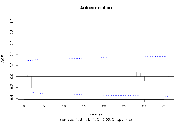
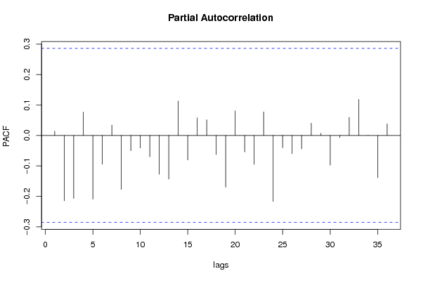
Title produced by software

(Partial) Autocorrelation Function

Date of computation

Fri, 27 Nov 2009 05:17:11 -0700

Cite this page as follows

Statistical Computations at FreeStatistics.org, Office for Research Development and Education, URL https://freestatistics.org/blog/index.php?v=date/2009/Nov/27/t1259324295elajdb0472i2r9q.htm/, Retrieved Mon, 29 Apr 2024 07:17:28 +0000

Statistical Computations at FreeStatistics.org, Office for Research Development and Education, URL https://freestatistics.org/blog/index.php?pk=60624, Retrieved Mon, 29 Apr 2024 07:17:28 +0000

QR Codes:

Paste this QR Code to cite your computation.

Original text written by user:

IsPrivate?

No (this computation is public)

User-defined keywords

Estimated Impact

165

Family? (F = Feedback message, R = changed R code, M = changed R Module, P = changed Parameters, D = changed Data)

-     [Univariate Explorative Data Analysis] [Run Sequence gebo...] [2008-12-12 13:32:37] [76963dc1903f0f612b6153510a3818cf]
- R  D  [Univariate Explorative Data Analysis] [Run Sequence gebo...] [2008-12-17 12:14:40] [76963dc1903f0f612b6153510a3818cf]
-         [Univariate Explorative Data Analysis] [Run Sequence Plot...] [2008-12-22 18:19:51] [1ce0d16c8f4225c977b42c8fa93bc163]
- RMP       [(Partial) Autocorrelation Function] [Identifying Integ...] [2009-11-22 12:16:10] [b98453cac15ba1066b407e146608df68]
-   PD          [(Partial) Autocorrelation Function] [Ws 8 autocorrelat...] [2009-11-27 12:17:11] [51d49d3536f6a59f2486a67bf50b2759] [Current]
- RMPD            [Univariate Explorative Data Analysis] [Paper Y3 EDA] [2009-12-14 09:17:22] [4637f404ac59dfaba4ecf14efa20abbd] 
- RMPD            [Univariate Explorative Data Analysis] [Paper Y3 Autocor ...] [2009-12-14 09:17:22] [4637f404ac59dfaba4ecf14efa20abbd] 
- RMPD            [Univariate Explorative Data Analysis] [Paper Y3 autocor ...] [2009-12-14 09:17:22] [4637f404ac59dfaba4ecf14efa20abbd] 
-   PD            [(Partial) Autocorrelation Function] [Paper Y3 autocor ...] [2009-12-14 10:04:29] [4637f404ac59dfaba4ecf14efa20abbd] 
-   PD            [(Partial) Autocorrelation Function] [Paper Y3 d=1 D=0] [2009-12-14 10:16:18] [4637f404ac59dfaba4ecf14efa20abbd] 
-   PD            [(Partial) Autocorrelation Function] [Paper Y3 D=d=1] [2009-12-14 10:36:30] [4637f404ac59dfaba4ecf14efa20abbd] 
- RMP               [Variance Reduction Matrix] [Paper Y3 variance...] [2009-12-17 09:42:04] [4637f404ac59dfaba4ecf14efa20abbd] 
- RMP               [Standard Deviation-Mean Plot] [Paper SdMP Y3 ] [2009-12-17 10:18:03] [4637f404ac59dfaba4ecf14efa20abbd] 

Feedback Forum

Post a new message

Dataseries X:

Download CSV

Histogram

Boxplots

Summary of computational transaction
Raw Input	view raw input (R code)
Raw Output	view raw output of R engine
Computing time	1 seconds
R Server	'Gwilym Jenkins' @ 72.249.127.135

\begin{tabular}{lllllllll}
\hline
Summary of computational transaction \tabularnewline
Raw Input & view raw input (R code)  \tabularnewline
Raw Output & view raw output of R engine  \tabularnewline
Computing time & 1 seconds \tabularnewline
R Server & 'Gwilym Jenkins' @ 72.249.127.135 \tabularnewline
\hline
\end{tabular}
%Source: https://freestatistics.org/blog/index.php?pk=60624&T=0

[TABLE]
[ROW][C]Summary of computational transaction[/C][/ROW]
[ROW][C]Raw Input[/C][C]view raw input (R code) [/C][/ROW]
[ROW][C]Raw Output[/C][C]view raw output of R engine [/C][/ROW]
[ROW][C]Computing time[/C][C]1 seconds[/C][/ROW]
[ROW][C]R Server[/C][C]'Gwilym Jenkins' @ 72.249.127.135[/C][/ROW]
[/TABLE]
Source: https://freestatistics.org/blog/index.php?pk=60624&T=0

Globally Unique Identifier (entire table): ba.freestatistics.org/blog/index.php?pk=60624&T=0

As an alternative you can also use a QR Code:

The GUIDs for individual cells are displayed in the table below:

Summary of computational transaction
Raw Input	view raw input (R code)
Raw Output	view raw output of R engine
Computing time	1 seconds
R Server	'Gwilym Jenkins' @ 72.249.127.135

Autocorrelation Function
Time lag k	ACF(k)	T-STAT	P-value
1	0.014093	0.0966	0.46172
2	-0.214508	-1.4706	0.074032
3	-0.204166	-1.3997	0.084086
4	0.117981	0.8088	0.211342
5	-0.106341	-0.729	0.234799
6	-0.079424	-0.5445	0.294334
7	0.056224	0.3855	0.35082
8	-0.037708	-0.2585	0.398571
9	-0.049837	-0.3417	0.367064
10	-0.005173	-0.0355	0.48593
11	0.054295	0.3722	0.355697
12	-0.096369	-0.6607	0.256025
13	-0.08789	-0.6025	0.274854
14	0.184163	1.2626	0.106489
15	0.047851	0.328	0.372167
16	0.026994	0.1851	0.42699
17	-0.017939	-0.123	0.451322
18	0.021203	0.1454	0.442523
19	-0.210633	-1.444	0.077682
20	0.051598	0.3537	0.362559
21	0.07161	0.4909	0.312879
22	-0.024978	-0.1712	0.432385
23	-0.027406	-0.1879	0.425887
24	-0.085228	-0.5843	0.280909
25	0.037455	0.2568	0.399235
26	-0.058608	-0.4018	0.344828
27	0.077228	0.5295	0.299492
28	0.071757	0.4919	0.312526
29	0.059837	0.4102	0.341753
30	-0.087694	-0.6012	0.275299
31	0.012245	0.0839	0.466729
32	0.114782	0.7869	0.217644
33	0.034319	0.2353	0.407508
34	-0.040598	-0.2783	0.390993
35	-0.16627	-1.1399	0.130054
36	-0.001553	-0.0106	0.495776

\begin{tabular}{lllllllll}
\hline
Autocorrelation Function \tabularnewline
Time lag k & ACF(k) & T-STAT & P-value \tabularnewline
1 & 0.014093 & 0.0966 & 0.46172 \tabularnewline
2 & -0.214508 & -1.4706 & 0.074032 \tabularnewline
3 & -0.204166 & -1.3997 & 0.084086 \tabularnewline
4 & 0.117981 & 0.8088 & 0.211342 \tabularnewline
5 & -0.106341 & -0.729 & 0.234799 \tabularnewline
6 & -0.079424 & -0.5445 & 0.294334 \tabularnewline
7 & 0.056224 & 0.3855 & 0.35082 \tabularnewline
8 & -0.037708 & -0.2585 & 0.398571 \tabularnewline
9 & -0.049837 & -0.3417 & 0.367064 \tabularnewline
10 & -0.005173 & -0.0355 & 0.48593 \tabularnewline
11 & 0.054295 & 0.3722 & 0.355697 \tabularnewline
12 & -0.096369 & -0.6607 & 0.256025 \tabularnewline
13 & -0.08789 & -0.6025 & 0.274854 \tabularnewline
14 & 0.184163 & 1.2626 & 0.106489 \tabularnewline
15 & 0.047851 & 0.328 & 0.372167 \tabularnewline
16 & 0.026994 & 0.1851 & 0.42699 \tabularnewline
17 & -0.017939 & -0.123 & 0.451322 \tabularnewline
18 & 0.021203 & 0.1454 & 0.442523 \tabularnewline
19 & -0.210633 & -1.444 & 0.077682 \tabularnewline
20 & 0.051598 & 0.3537 & 0.362559 \tabularnewline
21 & 0.07161 & 0.4909 & 0.312879 \tabularnewline
22 & -0.024978 & -0.1712 & 0.432385 \tabularnewline
23 & -0.027406 & -0.1879 & 0.425887 \tabularnewline
24 & -0.085228 & -0.5843 & 0.280909 \tabularnewline
25 & 0.037455 & 0.2568 & 0.399235 \tabularnewline
26 & -0.058608 & -0.4018 & 0.344828 \tabularnewline
27 & 0.077228 & 0.5295 & 0.299492 \tabularnewline
28 & 0.071757 & 0.4919 & 0.312526 \tabularnewline
29 & 0.059837 & 0.4102 & 0.341753 \tabularnewline
30 & -0.087694 & -0.6012 & 0.275299 \tabularnewline
31 & 0.012245 & 0.0839 & 0.466729 \tabularnewline
32 & 0.114782 & 0.7869 & 0.217644 \tabularnewline
33 & 0.034319 & 0.2353 & 0.407508 \tabularnewline
34 & -0.040598 & -0.2783 & 0.390993 \tabularnewline
35 & -0.16627 & -1.1399 & 0.130054 \tabularnewline
36 & -0.001553 & -0.0106 & 0.495776 \tabularnewline
\hline
\end{tabular}
%Source: https://freestatistics.org/blog/index.php?pk=60624&T=1

[TABLE]
[ROW][C]Autocorrelation Function[/C][/ROW]
[ROW][C]Time lag k[/C][C]ACF(k)[/C][C]T-STAT[/C][C]P-value[/C][/ROW]
[ROW][C]1[/C][C]0.014093[/C][C]0.0966[/C][C]0.46172[/C][/ROW]
[ROW][C]2[/C][C]-0.214508[/C][C]-1.4706[/C][C]0.074032[/C][/ROW]
[ROW][C]3[/C][C]-0.204166[/C][C]-1.3997[/C][C]0.084086[/C][/ROW]
[ROW][C]4[/C][C]0.117981[/C][C]0.8088[/C][C]0.211342[/C][/ROW]
[ROW][C]5[/C][C]-0.106341[/C][C]-0.729[/C][C]0.234799[/C][/ROW]
[ROW][C]6[/C][C]-0.079424[/C][C]-0.5445[/C][C]0.294334[/C][/ROW]
[ROW][C]7[/C][C]0.056224[/C][C]0.3855[/C][C]0.35082[/C][/ROW]
[ROW][C]8[/C][C]-0.037708[/C][C]-0.2585[/C][C]0.398571[/C][/ROW]
[ROW][C]9[/C][C]-0.049837[/C][C]-0.3417[/C][C]0.367064[/C][/ROW]
[ROW][C]10[/C][C]-0.005173[/C][C]-0.0355[/C][C]0.48593[/C][/ROW]
[ROW][C]11[/C][C]0.054295[/C][C]0.3722[/C][C]0.355697[/C][/ROW]
[ROW][C]12[/C][C]-0.096369[/C][C]-0.6607[/C][C]0.256025[/C][/ROW]
[ROW][C]13[/C][C]-0.08789[/C][C]-0.6025[/C][C]0.274854[/C][/ROW]
[ROW][C]14[/C][C]0.184163[/C][C]1.2626[/C][C]0.106489[/C][/ROW]
[ROW][C]15[/C][C]0.047851[/C][C]0.328[/C][C]0.372167[/C][/ROW]
[ROW][C]16[/C][C]0.026994[/C][C]0.1851[/C][C]0.42699[/C][/ROW]
[ROW][C]17[/C][C]-0.017939[/C][C]-0.123[/C][C]0.451322[/C][/ROW]
[ROW][C]18[/C][C]0.021203[/C][C]0.1454[/C][C]0.442523[/C][/ROW]
[ROW][C]19[/C][C]-0.210633[/C][C]-1.444[/C][C]0.077682[/C][/ROW]
[ROW][C]20[/C][C]0.051598[/C][C]0.3537[/C][C]0.362559[/C][/ROW]
[ROW][C]21[/C][C]0.07161[/C][C]0.4909[/C][C]0.312879[/C][/ROW]
[ROW][C]22[/C][C]-0.024978[/C][C]-0.1712[/C][C]0.432385[/C][/ROW]
[ROW][C]23[/C][C]-0.027406[/C][C]-0.1879[/C][C]0.425887[/C][/ROW]
[ROW][C]24[/C][C]-0.085228[/C][C]-0.5843[/C][C]0.280909[/C][/ROW]
[ROW][C]25[/C][C]0.037455[/C][C]0.2568[/C][C]0.399235[/C][/ROW]
[ROW][C]26[/C][C]-0.058608[/C][C]-0.4018[/C][C]0.344828[/C][/ROW]
[ROW][C]27[/C][C]0.077228[/C][C]0.5295[/C][C]0.299492[/C][/ROW]
[ROW][C]28[/C][C]0.071757[/C][C]0.4919[/C][C]0.312526[/C][/ROW]
[ROW][C]29[/C][C]0.059837[/C][C]0.4102[/C][C]0.341753[/C][/ROW]
[ROW][C]30[/C][C]-0.087694[/C][C]-0.6012[/C][C]0.275299[/C][/ROW]
[ROW][C]31[/C][C]0.012245[/C][C]0.0839[/C][C]0.466729[/C][/ROW]
[ROW][C]32[/C][C]0.114782[/C][C]0.7869[/C][C]0.217644[/C][/ROW]
[ROW][C]33[/C][C]0.034319[/C][C]0.2353[/C][C]0.407508[/C][/ROW]
[ROW][C]34[/C][C]-0.040598[/C][C]-0.2783[/C][C]0.390993[/C][/ROW]
[ROW][C]35[/C][C]-0.16627[/C][C]-1.1399[/C][C]0.130054[/C][/ROW]
[ROW][C]36[/C][C]-0.001553[/C][C]-0.0106[/C][C]0.495776[/C][/ROW]
[/TABLE]
Source: https://freestatistics.org/blog/index.php?pk=60624&T=1

Globally Unique Identifier (entire table): ba.freestatistics.org/blog/index.php?pk=60624&T=1

As an alternative you can also use a QR Code:

The GUIDs for individual cells are displayed in the table below:

Autocorrelation Function
Time lag k	ACF(k)	T-STAT	P-value
1	0.014093	0.0966	0.46172
2	-0.214508	-1.4706	0.074032
3	-0.204166	-1.3997	0.084086
4	0.117981	0.8088	0.211342
5	-0.106341	-0.729	0.234799
6	-0.079424	-0.5445	0.294334
7	0.056224	0.3855	0.35082
8	-0.037708	-0.2585	0.398571
9	-0.049837	-0.3417	0.367064
10	-0.005173	-0.0355	0.48593
11	0.054295	0.3722	0.355697
12	-0.096369	-0.6607	0.256025
13	-0.08789	-0.6025	0.274854
14	0.184163	1.2626	0.106489
15	0.047851	0.328	0.372167
16	0.026994	0.1851	0.42699
17	-0.017939	-0.123	0.451322
18	0.021203	0.1454	0.442523
19	-0.210633	-1.444	0.077682
20	0.051598	0.3537	0.362559
21	0.07161	0.4909	0.312879
22	-0.024978	-0.1712	0.432385
23	-0.027406	-0.1879	0.425887
24	-0.085228	-0.5843	0.280909
25	0.037455	0.2568	0.399235
26	-0.058608	-0.4018	0.344828
27	0.077228	0.5295	0.299492
28	0.071757	0.4919	0.312526
29	0.059837	0.4102	0.341753
30	-0.087694	-0.6012	0.275299
31	0.012245	0.0839	0.466729
32	0.114782	0.7869	0.217644
33	0.034319	0.2353	0.407508
34	-0.040598	-0.2783	0.390993
35	-0.16627	-1.1399	0.130054
36	-0.001553	-0.0106	0.495776

Partial Autocorrelation Function
Time lag k	PACF(k)	T-STAT	P-value
1	0.014093	0.0966	0.46172
2	-0.214749	-1.4722	0.07381
3	-0.207055	-1.4195	0.081177
4	0.076699	0.5258	0.300742
5	-0.209213	-1.4343	0.079055
6	-0.094684	-0.6491	0.259709
7	0.034103	0.2338	0.408078
8	-0.177531	-1.2171	0.114823
9	-0.050307	-0.3449	0.365859
10	-0.041533	-0.2847	0.388549
11	-0.070283	-0.4818	0.316078
12	-0.12759	-0.8747	0.193089
13	-0.143387	-0.983	0.165317
14	0.112994	0.7747	0.221213
15	-0.080818	-0.5541	0.291081
16	0.05808	0.3982	0.346151
17	0.051245	0.3513	0.363459
18	-0.062947	-0.4315	0.334024
19	-0.170237	-1.1671	0.124531
20	0.080904	0.5546	0.290882
21	-0.054306	-0.3723	0.35567
22	-0.094993	-0.6512	0.259032
23	0.077583	0.5319	0.298655
24	-0.216732	-1.4858	0.072
25	-0.040769	-0.2795	0.390546
26	-0.059946	-0.411	0.341481
27	-0.044065	-0.3021	0.381956
28	0.040232	0.2758	0.391949
29	0.007245	0.0497	0.480297
30	-0.097532	-0.6686	0.253496
31	-0.006855	-0.047	0.481357
32	0.059748	0.4096	0.341975
33	0.118653	0.8134	0.210033
34	-0.001012	-0.0069	0.497248
35	-0.138745	-0.9512	0.173187
36	0.03812	0.2613	0.397487

\begin{tabular}{lllllllll}
\hline
Partial Autocorrelation Function \tabularnewline
Time lag k & PACF(k) & T-STAT & P-value \tabularnewline
1 & 0.014093 & 0.0966 & 0.46172 \tabularnewline
2 & -0.214749 & -1.4722 & 0.07381 \tabularnewline
3 & -0.207055 & -1.4195 & 0.081177 \tabularnewline
4 & 0.076699 & 0.5258 & 0.300742 \tabularnewline
5 & -0.209213 & -1.4343 & 0.079055 \tabularnewline
6 & -0.094684 & -0.6491 & 0.259709 \tabularnewline
7 & 0.034103 & 0.2338 & 0.408078 \tabularnewline
8 & -0.177531 & -1.2171 & 0.114823 \tabularnewline
9 & -0.050307 & -0.3449 & 0.365859 \tabularnewline
10 & -0.041533 & -0.2847 & 0.388549 \tabularnewline
11 & -0.070283 & -0.4818 & 0.316078 \tabularnewline
12 & -0.12759 & -0.8747 & 0.193089 \tabularnewline
13 & -0.143387 & -0.983 & 0.165317 \tabularnewline
14 & 0.112994 & 0.7747 & 0.221213 \tabularnewline
15 & -0.080818 & -0.5541 & 0.291081 \tabularnewline
16 & 0.05808 & 0.3982 & 0.346151 \tabularnewline
17 & 0.051245 & 0.3513 & 0.363459 \tabularnewline
18 & -0.062947 & -0.4315 & 0.334024 \tabularnewline
19 & -0.170237 & -1.1671 & 0.124531 \tabularnewline
20 & 0.080904 & 0.5546 & 0.290882 \tabularnewline
21 & -0.054306 & -0.3723 & 0.35567 \tabularnewline
22 & -0.094993 & -0.6512 & 0.259032 \tabularnewline
23 & 0.077583 & 0.5319 & 0.298655 \tabularnewline
24 & -0.216732 & -1.4858 & 0.072 \tabularnewline
25 & -0.040769 & -0.2795 & 0.390546 \tabularnewline
26 & -0.059946 & -0.411 & 0.341481 \tabularnewline
27 & -0.044065 & -0.3021 & 0.381956 \tabularnewline
28 & 0.040232 & 0.2758 & 0.391949 \tabularnewline
29 & 0.007245 & 0.0497 & 0.480297 \tabularnewline
30 & -0.097532 & -0.6686 & 0.253496 \tabularnewline
31 & -0.006855 & -0.047 & 0.481357 \tabularnewline
32 & 0.059748 & 0.4096 & 0.341975 \tabularnewline
33 & 0.118653 & 0.8134 & 0.210033 \tabularnewline
34 & -0.001012 & -0.0069 & 0.497248 \tabularnewline
35 & -0.138745 & -0.9512 & 0.173187 \tabularnewline
36 & 0.03812 & 0.2613 & 0.397487 \tabularnewline
\hline
\end{tabular}
%Source: https://freestatistics.org/blog/index.php?pk=60624&T=2

[TABLE]
[ROW][C]Partial Autocorrelation Function[/C][/ROW]
[ROW][C]Time lag k[/C][C]PACF(k)[/C][C]T-STAT[/C][C]P-value[/C][/ROW]
[ROW][C]1[/C][C]0.014093[/C][C]0.0966[/C][C]0.46172[/C][/ROW]
[ROW][C]2[/C][C]-0.214749[/C][C]-1.4722[/C][C]0.07381[/C][/ROW]
[ROW][C]3[/C][C]-0.207055[/C][C]-1.4195[/C][C]0.081177[/C][/ROW]
[ROW][C]4[/C][C]0.076699[/C][C]0.5258[/C][C]0.300742[/C][/ROW]
[ROW][C]5[/C][C]-0.209213[/C][C]-1.4343[/C][C]0.079055[/C][/ROW]
[ROW][C]6[/C][C]-0.094684[/C][C]-0.6491[/C][C]0.259709[/C][/ROW]
[ROW][C]7[/C][C]0.034103[/C][C]0.2338[/C][C]0.408078[/C][/ROW]
[ROW][C]8[/C][C]-0.177531[/C][C]-1.2171[/C][C]0.114823[/C][/ROW]
[ROW][C]9[/C][C]-0.050307[/C][C]-0.3449[/C][C]0.365859[/C][/ROW]
[ROW][C]10[/C][C]-0.041533[/C][C]-0.2847[/C][C]0.388549[/C][/ROW]
[ROW][C]11[/C][C]-0.070283[/C][C]-0.4818[/C][C]0.316078[/C][/ROW]
[ROW][C]12[/C][C]-0.12759[/C][C]-0.8747[/C][C]0.193089[/C][/ROW]
[ROW][C]13[/C][C]-0.143387[/C][C]-0.983[/C][C]0.165317[/C][/ROW]
[ROW][C]14[/C][C]0.112994[/C][C]0.7747[/C][C]0.221213[/C][/ROW]
[ROW][C]15[/C][C]-0.080818[/C][C]-0.5541[/C][C]0.291081[/C][/ROW]
[ROW][C]16[/C][C]0.05808[/C][C]0.3982[/C][C]0.346151[/C][/ROW]
[ROW][C]17[/C][C]0.051245[/C][C]0.3513[/C][C]0.363459[/C][/ROW]
[ROW][C]18[/C][C]-0.062947[/C][C]-0.4315[/C][C]0.334024[/C][/ROW]
[ROW][C]19[/C][C]-0.170237[/C][C]-1.1671[/C][C]0.124531[/C][/ROW]
[ROW][C]20[/C][C]0.080904[/C][C]0.5546[/C][C]0.290882[/C][/ROW]
[ROW][C]21[/C][C]-0.054306[/C][C]-0.3723[/C][C]0.35567[/C][/ROW]
[ROW][C]22[/C][C]-0.094993[/C][C]-0.6512[/C][C]0.259032[/C][/ROW]
[ROW][C]23[/C][C]0.077583[/C][C]0.5319[/C][C]0.298655[/C][/ROW]
[ROW][C]24[/C][C]-0.216732[/C][C]-1.4858[/C][C]0.072[/C][/ROW]
[ROW][C]25[/C][C]-0.040769[/C][C]-0.2795[/C][C]0.390546[/C][/ROW]
[ROW][C]26[/C][C]-0.059946[/C][C]-0.411[/C][C]0.341481[/C][/ROW]
[ROW][C]27[/C][C]-0.044065[/C][C]-0.3021[/C][C]0.381956[/C][/ROW]
[ROW][C]28[/C][C]0.040232[/C][C]0.2758[/C][C]0.391949[/C][/ROW]
[ROW][C]29[/C][C]0.007245[/C][C]0.0497[/C][C]0.480297[/C][/ROW]
[ROW][C]30[/C][C]-0.097532[/C][C]-0.6686[/C][C]0.253496[/C][/ROW]
[ROW][C]31[/C][C]-0.006855[/C][C]-0.047[/C][C]0.481357[/C][/ROW]
[ROW][C]32[/C][C]0.059748[/C][C]0.4096[/C][C]0.341975[/C][/ROW]
[ROW][C]33[/C][C]0.118653[/C][C]0.8134[/C][C]0.210033[/C][/ROW]
[ROW][C]34[/C][C]-0.001012[/C][C]-0.0069[/C][C]0.497248[/C][/ROW]
[ROW][C]35[/C][C]-0.138745[/C][C]-0.9512[/C][C]0.173187[/C][/ROW]
[ROW][C]36[/C][C]0.03812[/C][C]0.2613[/C][C]0.397487[/C][/ROW]
[/TABLE]
Source: https://freestatistics.org/blog/index.php?pk=60624&T=2

Globally Unique Identifier (entire table): ba.freestatistics.org/blog/index.php?pk=60624&T=2

As an alternative you can also use a QR Code:

The GUIDs for individual cells are displayed in the table below:

Partial Autocorrelation Function
Time lag k	PACF(k)	T-STAT	P-value
1	0.014093	0.0966	0.46172
2	-0.214749	-1.4722	0.07381
3	-0.207055	-1.4195	0.081177
4	0.076699	0.5258	0.300742
5	-0.209213	-1.4343	0.079055
6	-0.094684	-0.6491	0.259709
7	0.034103	0.2338	0.408078
8	-0.177531	-1.2171	0.114823
9	-0.050307	-0.3449	0.365859
10	-0.041533	-0.2847	0.388549
11	-0.070283	-0.4818	0.316078
12	-0.12759	-0.8747	0.193089
13	-0.143387	-0.983	0.165317
14	0.112994	0.7747	0.221213
15	-0.080818	-0.5541	0.291081
16	0.05808	0.3982	0.346151
17	0.051245	0.3513	0.363459
18	-0.062947	-0.4315	0.334024
19	-0.170237	-1.1671	0.124531
20	0.080904	0.5546	0.290882
21	-0.054306	-0.3723	0.35567
22	-0.094993	-0.6512	0.259032
23	0.077583	0.5319	0.298655
24	-0.216732	-1.4858	0.072
25	-0.040769	-0.2795	0.390546
26	-0.059946	-0.411	0.341481
27	-0.044065	-0.3021	0.381956
28	0.040232	0.2758	0.391949
29	0.007245	0.0497	0.480297
30	-0.097532	-0.6686	0.253496
31	-0.006855	-0.047	0.481357
32	0.059748	0.4096	0.341975
33	0.118653	0.8134	0.210033
34	-0.001012	-0.0069	0.497248
35	-0.138745	-0.9512	0.173187
36	0.03812	0.2613	0.397487

Figure 1

PNG link

Postscript link

PDF link

Figure 2

PNG link

Postscript link

PDF link

Parameters (Session):

par1 = 36 ; par2 = 1 ; par3 = 1 ; par4 = 1 ; par5 = 12 ; par6 = MA ; par7 = 0.95 ;

Parameters (R input):

par1 = 36 ; par2 = 1 ; par3 = 1 ; par4 = 1 ; par5 = 12 ; par6 = MA ; par7 = 0.95 ;

R code (references can be found in the software module):

if (par1 == 'Default') {
par1 = 10*log10(length(x))
} else {
par1 <- as.numeric(par1)
}
par2 <- as.numeric(par2)
par3 <- as.numeric(par3)
par4 <- as.numeric(par4)
par5 <- as.numeric(par5)
if (par6 == 'White Noise') par6 <- 'white' else par6 <- 'ma'
par7 <- as.numeric(par7)
if (par2 == 0) {
x <- log(x)
} else {
x <- (x ^ par2 - 1) / par2
}
if (par3 > 0) x <- diff(x,lag=1,difference=par3)
if (par4 > 0) x <- diff(x,lag=par5,difference=par4)
bitmap(file='pic1.png')
racf <- acf(x, par1, main='Autocorrelation', xlab='time lag', ylab='ACF', ci.type=par6, ci=par7, sub=paste('(lambda=',par2,', d=',par3,', D=',par4,', CI=', par7, ', CI type=',par6,')',sep=''))
dev.off()
bitmap(file='pic2.png')
rpacf <- pacf(x,par1,main='Partial Autocorrelation',xlab='lags',ylab='PACF')
dev.off()
(myacf <- c(racf$acf))
(mypacf <- c(rpacf$acf))
lengthx <- length(x)
sqrtn <- sqrt(lengthx)
load(file='createtable')
a<-table.start()
a<-table.row.start(a)
a<-table.element(a,'Autocorrelation Function',4,TRUE)
a<-table.row.end(a)
a<-table.row.start(a)
a<-table.element(a,'Time lag k',header=TRUE)
a<-table.element(a,hyperlink('basics.htm','ACF(k)','click here for more information about the Autocorrelation Function'),header=TRUE)
a<-table.element(a,'T-STAT',header=TRUE)
a<-table.element(a,'P-value',header=TRUE)
a<-table.row.end(a)
for (i in 2:(par1+1)) {
a<-table.row.start(a)
a<-table.element(a,i-1,header=TRUE)
a<-table.element(a,round(myacf[i],6))
mytstat <- myacf[i]*sqrtn
a<-table.element(a,round(mytstat,4))
a<-table.element(a,round(1-pt(abs(mytstat),lengthx),6))
a<-table.row.end(a)
}
a<-table.end(a)
table.save(a,file='mytable.tab')
a<-table.start()
a<-table.row.start(a)
a<-table.element(a,'Partial Autocorrelation Function',4,TRUE)
a<-table.row.end(a)
a<-table.row.start(a)
a<-table.element(a,'Time lag k',header=TRUE)
a<-table.element(a,hyperlink('basics.htm','PACF(k)','click here for more information about the Partial Autocorrelation Function'),header=TRUE)
a<-table.element(a,'T-STAT',header=TRUE)
a<-table.element(a,'P-value',header=TRUE)
a<-table.row.end(a)
for (i in 1:par1) {
a<-table.row.start(a)
a<-table.element(a,i,header=TRUE)
a<-table.element(a,round(mypacf[i],6))
mytstat <- mypacf[i]*sqrtn
a<-table.element(a,round(mytstat,4))
a<-table.element(a,round(1-pt(abs(mytstat),lengthx),6))
a<-table.row.end(a)
}
a<-table.end(a)
table.save(a,file='mytable1.tab')

Free Statistics

Description of Statistical Computation

Tree of Dependent Computations

Dataset

Tables (Output of Computation)

Figures (Output of Computation)

Input Parameters & R Code