Repository of Reproducible Computations

Free Statistics

of Irreproducible Research!

Author's title

Author

*The author of this computation has been verified*

R Software Module

rwasp_autocorrelation.wasp

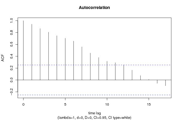
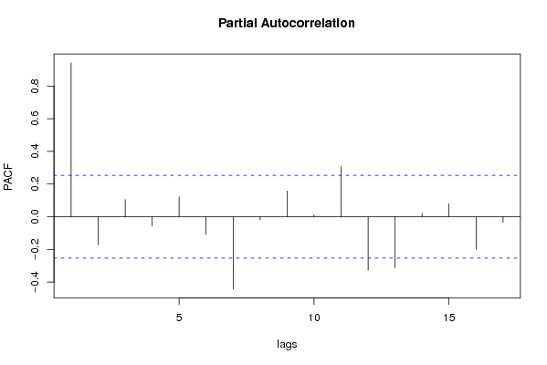
Title produced by software

(Partial) Autocorrelation Function

Date of computation

Fri, 27 Nov 2009 06:34:22 -0700

Cite this page as follows

Statistical Computations at FreeStatistics.org, Office for Research Development and Education, URL https://freestatistics.org/blog/index.php?v=date/2009/Nov/27/t1259329020hdp72bjkcwm6qag.htm/, Retrieved Sun, 28 Apr 2024 19:02:54 +0000

Statistical Computations at FreeStatistics.org, Office for Research Development and Education, URL https://freestatistics.org/blog/index.php?pk=60743, Retrieved Sun, 28 Apr 2024 19:02:54 +0000

QR Codes:

Paste this QR Code to cite your computation.

Original text written by user:

IsPrivate?

No (this computation is public)

User-defined keywords

shwws8

Estimated Impact

201

Family? (F = Feedback message, R = changed R code, M = changed R Module, P = changed Parameters, D = changed Data)

-     [Multiple Regression] [Q1 The Seatbeltlaw] [2007-11-14 19:27:43] [8cd6641b921d30ebe00b648d1481bba0]
- RMPD  [Multiple Regression] [Seatbelt] [2009-11-12 13:54:52] [b98453cac15ba1066b407e146608df68]
-   PD    [Multiple Regression] [W7] [2009-11-18 21:32:41] [315ba876df544ad397193b5931d5f354]
- RMPD        [(Partial) Autocorrelation Function] [] [2009-11-27 13:34:22] [efdfe680cd785c4af09f858b30f777ec] [Current]
-   P           [(Partial) Autocorrelation Function] [workshop 8] [2009-11-28 12:11:27] [eaf42bcf5162b5692bb3c7f9d4636222] 
-   P           [(Partial) Autocorrelation Function] [] [2009-12-02 14:48:19] [5482608004c1d7bbf873930172393a2d] 
-   P           [(Partial) Autocorrelation Function] [] [2009-12-02 14:58:25] [5482608004c1d7bbf873930172393a2d] 
-   P           [(Partial) Autocorrelation Function] [ws8: acf verbetering] [2009-12-04 19:00:06] [bd8e774728cf1f2f4e6868fd314defe3] 
- RMP           [ARIMA Forecasting] [ARIMA Forecast] [2009-12-11 12:59:37] [5482608004c1d7bbf873930172393a2d] 

Feedback Forum

Post a new message

Dataseries X:

Download CSV

Histogram

Boxplots

Summary of computational transaction
Raw Input	view raw input (R code)
Raw Output	view raw output of R engine
Computing time	1 seconds
R Server	'Gwilym Jenkins' @ 72.249.127.135

\begin{tabular}{lllllllll}
\hline
Summary of computational transaction \tabularnewline
Raw Input & view raw input (R code)  \tabularnewline
Raw Output & view raw output of R engine  \tabularnewline
Computing time & 1 seconds \tabularnewline
R Server & 'Gwilym Jenkins' @ 72.249.127.135 \tabularnewline
\hline
\end{tabular}
%Source: https://freestatistics.org/blog/index.php?pk=60743&T=0

[TABLE]
[ROW][C]Summary of computational transaction[/C][/ROW]
[ROW][C]Raw Input[/C][C]view raw input (R code) [/C][/ROW]
[ROW][C]Raw Output[/C][C]view raw output of R engine [/C][/ROW]
[ROW][C]Computing time[/C][C]1 seconds[/C][/ROW]
[ROW][C]R Server[/C][C]'Gwilym Jenkins' @ 72.249.127.135[/C][/ROW]
[/TABLE]
Source: https://freestatistics.org/blog/index.php?pk=60743&T=0

Globally Unique Identifier (entire table): ba.freestatistics.org/blog/index.php?pk=60743&T=0

As an alternative you can also use a QR Code:

The GUIDs for individual cells are displayed in the table below:

Summary of computational transaction
Raw Input	view raw input (R code)
Raw Output	view raw output of R engine
Computing time	1 seconds
R Server	'Gwilym Jenkins' @ 72.249.127.135

Autocorrelation Function
Time lag k	ACF(k)	T-STAT	P-value
1	0.941403	7.2921	0
2	0.866809	6.7143	0
3	0.806212	6.2449	0
4	0.74743	5.7896	0
5	0.703624	5.4502	0
6	0.656437	5.0847	2e-06
7	0.559228	4.3318	2.9e-05
8	0.454536	3.5208	0.000414
9	0.378883	2.9348	0.002362
10	0.316079	2.4483	0.008646
11	0.293258	2.2716	0.013356
12	0.255991	1.9829	0.025981
13	0.166381	1.2888	0.101211
14	0.074366	0.576	0.283372
15	0.009734	0.0754	0.470073
16	-0.056243	-0.4357	0.332324
17	-0.097273	-0.7535	0.227056

\begin{tabular}{lllllllll}
\hline
Autocorrelation Function \tabularnewline
Time lag k & ACF(k) & T-STAT & P-value \tabularnewline
1 & 0.941403 & 7.2921 & 0 \tabularnewline
2 & 0.866809 & 6.7143 & 0 \tabularnewline
3 & 0.806212 & 6.2449 & 0 \tabularnewline
4 & 0.74743 & 5.7896 & 0 \tabularnewline
5 & 0.703624 & 5.4502 & 0 \tabularnewline
6 & 0.656437 & 5.0847 & 2e-06 \tabularnewline
7 & 0.559228 & 4.3318 & 2.9e-05 \tabularnewline
8 & 0.454536 & 3.5208 & 0.000414 \tabularnewline
9 & 0.378883 & 2.9348 & 0.002362 \tabularnewline
10 & 0.316079 & 2.4483 & 0.008646 \tabularnewline
11 & 0.293258 & 2.2716 & 0.013356 \tabularnewline
12 & 0.255991 & 1.9829 & 0.025981 \tabularnewline
13 & 0.166381 & 1.2888 & 0.101211 \tabularnewline
14 & 0.074366 & 0.576 & 0.283372 \tabularnewline
15 & 0.009734 & 0.0754 & 0.470073 \tabularnewline
16 & -0.056243 & -0.4357 & 0.332324 \tabularnewline
17 & -0.097273 & -0.7535 & 0.227056 \tabularnewline
\hline
\end{tabular}
%Source: https://freestatistics.org/blog/index.php?pk=60743&T=1

[TABLE]
[ROW][C]Autocorrelation Function[/C][/ROW]
[ROW][C]Time lag k[/C][C]ACF(k)[/C][C]T-STAT[/C][C]P-value[/C][/ROW]
[ROW][C]1[/C][C]0.941403[/C][C]7.2921[/C][C]0[/C][/ROW]
[ROW][C]2[/C][C]0.866809[/C][C]6.7143[/C][C]0[/C][/ROW]
[ROW][C]3[/C][C]0.806212[/C][C]6.2449[/C][C]0[/C][/ROW]
[ROW][C]4[/C][C]0.74743[/C][C]5.7896[/C][C]0[/C][/ROW]
[ROW][C]5[/C][C]0.703624[/C][C]5.4502[/C][C]0[/C][/ROW]
[ROW][C]6[/C][C]0.656437[/C][C]5.0847[/C][C]2e-06[/C][/ROW]
[ROW][C]7[/C][C]0.559228[/C][C]4.3318[/C][C]2.9e-05[/C][/ROW]
[ROW][C]8[/C][C]0.454536[/C][C]3.5208[/C][C]0.000414[/C][/ROW]
[ROW][C]9[/C][C]0.378883[/C][C]2.9348[/C][C]0.002362[/C][/ROW]
[ROW][C]10[/C][C]0.316079[/C][C]2.4483[/C][C]0.008646[/C][/ROW]
[ROW][C]11[/C][C]0.293258[/C][C]2.2716[/C][C]0.013356[/C][/ROW]
[ROW][C]12[/C][C]0.255991[/C][C]1.9829[/C][C]0.025981[/C][/ROW]
[ROW][C]13[/C][C]0.166381[/C][C]1.2888[/C][C]0.101211[/C][/ROW]
[ROW][C]14[/C][C]0.074366[/C][C]0.576[/C][C]0.283372[/C][/ROW]
[ROW][C]15[/C][C]0.009734[/C][C]0.0754[/C][C]0.470073[/C][/ROW]
[ROW][C]16[/C][C]-0.056243[/C][C]-0.4357[/C][C]0.332324[/C][/ROW]
[ROW][C]17[/C][C]-0.097273[/C][C]-0.7535[/C][C]0.227056[/C][/ROW]
[/TABLE]
Source: https://freestatistics.org/blog/index.php?pk=60743&T=1

Globally Unique Identifier (entire table): ba.freestatistics.org/blog/index.php?pk=60743&T=1

As an alternative you can also use a QR Code:

The GUIDs for individual cells are displayed in the table below:

Autocorrelation Function
Time lag k	ACF(k)	T-STAT	P-value
1	0.941403	7.2921	0
2	0.866809	6.7143	0
3	0.806212	6.2449	0
4	0.74743	5.7896	0
5	0.703624	5.4502	0
6	0.656437	5.0847	2e-06
7	0.559228	4.3318	2.9e-05
8	0.454536	3.5208	0.000414
9	0.378883	2.9348	0.002362
10	0.316079	2.4483	0.008646
11	0.293258	2.2716	0.013356
12	0.255991	1.9829	0.025981
13	0.166381	1.2888	0.101211
14	0.074366	0.576	0.283372
15	0.009734	0.0754	0.470073
16	-0.056243	-0.4357	0.332324
17	-0.097273	-0.7535	0.227056

Partial Autocorrelation Function
Time lag k	PACF(k)	T-STAT	P-value
1	0.941403	7.2921	0
2	-0.170807	-1.3231	0.095416
3	0.105153	0.8145	0.209287
4	-0.056129	-0.4348	0.332644
5	0.122005	0.945	0.174213
6	-0.106554	-0.8254	0.206218
7	-0.441554	-3.4203	0.000565
8	-0.018798	-0.1456	0.442361
9	0.157996	1.2238	0.1129
10	0.01346	0.1043	0.458655
11	0.307581	2.3825	0.01019
12	-0.327009	-2.533	0.006971
13	-0.312743	-2.4225	0.009225
14	0.021517	0.1667	0.434095
15	0.079403	0.6151	0.270422
16	-0.198673	-1.5389	0.064541
17	-0.035834	-0.2776	0.391148

\begin{tabular}{lllllllll}
\hline
Partial Autocorrelation Function \tabularnewline
Time lag k & PACF(k) & T-STAT & P-value \tabularnewline
1 & 0.941403 & 7.2921 & 0 \tabularnewline
2 & -0.170807 & -1.3231 & 0.095416 \tabularnewline
3 & 0.105153 & 0.8145 & 0.209287 \tabularnewline
4 & -0.056129 & -0.4348 & 0.332644 \tabularnewline
5 & 0.122005 & 0.945 & 0.174213 \tabularnewline
6 & -0.106554 & -0.8254 & 0.206218 \tabularnewline
7 & -0.441554 & -3.4203 & 0.000565 \tabularnewline
8 & -0.018798 & -0.1456 & 0.442361 \tabularnewline
9 & 0.157996 & 1.2238 & 0.1129 \tabularnewline
10 & 0.01346 & 0.1043 & 0.458655 \tabularnewline
11 & 0.307581 & 2.3825 & 0.01019 \tabularnewline
12 & -0.327009 & -2.533 & 0.006971 \tabularnewline
13 & -0.312743 & -2.4225 & 0.009225 \tabularnewline
14 & 0.021517 & 0.1667 & 0.434095 \tabularnewline
15 & 0.079403 & 0.6151 & 0.270422 \tabularnewline
16 & -0.198673 & -1.5389 & 0.064541 \tabularnewline
17 & -0.035834 & -0.2776 & 0.391148 \tabularnewline
\hline
\end{tabular}
%Source: https://freestatistics.org/blog/index.php?pk=60743&T=2

[TABLE]
[ROW][C]Partial Autocorrelation Function[/C][/ROW]
[ROW][C]Time lag k[/C][C]PACF(k)[/C][C]T-STAT[/C][C]P-value[/C][/ROW]
[ROW][C]1[/C][C]0.941403[/C][C]7.2921[/C][C]0[/C][/ROW]
[ROW][C]2[/C][C]-0.170807[/C][C]-1.3231[/C][C]0.095416[/C][/ROW]
[ROW][C]3[/C][C]0.105153[/C][C]0.8145[/C][C]0.209287[/C][/ROW]
[ROW][C]4[/C][C]-0.056129[/C][C]-0.4348[/C][C]0.332644[/C][/ROW]
[ROW][C]5[/C][C]0.122005[/C][C]0.945[/C][C]0.174213[/C][/ROW]
[ROW][C]6[/C][C]-0.106554[/C][C]-0.8254[/C][C]0.206218[/C][/ROW]
[ROW][C]7[/C][C]-0.441554[/C][C]-3.4203[/C][C]0.000565[/C][/ROW]
[ROW][C]8[/C][C]-0.018798[/C][C]-0.1456[/C][C]0.442361[/C][/ROW]
[ROW][C]9[/C][C]0.157996[/C][C]1.2238[/C][C]0.1129[/C][/ROW]
[ROW][C]10[/C][C]0.01346[/C][C]0.1043[/C][C]0.458655[/C][/ROW]
[ROW][C]11[/C][C]0.307581[/C][C]2.3825[/C][C]0.01019[/C][/ROW]
[ROW][C]12[/C][C]-0.327009[/C][C]-2.533[/C][C]0.006971[/C][/ROW]
[ROW][C]13[/C][C]-0.312743[/C][C]-2.4225[/C][C]0.009225[/C][/ROW]
[ROW][C]14[/C][C]0.021517[/C][C]0.1667[/C][C]0.434095[/C][/ROW]
[ROW][C]15[/C][C]0.079403[/C][C]0.6151[/C][C]0.270422[/C][/ROW]
[ROW][C]16[/C][C]-0.198673[/C][C]-1.5389[/C][C]0.064541[/C][/ROW]
[ROW][C]17[/C][C]-0.035834[/C][C]-0.2776[/C][C]0.391148[/C][/ROW]
[/TABLE]
Source: https://freestatistics.org/blog/index.php?pk=60743&T=2

Globally Unique Identifier (entire table): ba.freestatistics.org/blog/index.php?pk=60743&T=2

As an alternative you can also use a QR Code:

The GUIDs for individual cells are displayed in the table below:

Partial Autocorrelation Function
Time lag k	PACF(k)	T-STAT	P-value
1	0.941403	7.2921	0
2	-0.170807	-1.3231	0.095416
3	0.105153	0.8145	0.209287
4	-0.056129	-0.4348	0.332644
5	0.122005	0.945	0.174213
6	-0.106554	-0.8254	0.206218
7	-0.441554	-3.4203	0.000565
8	-0.018798	-0.1456	0.442361
9	0.157996	1.2238	0.1129
10	0.01346	0.1043	0.458655
11	0.307581	2.3825	0.01019
12	-0.327009	-2.533	0.006971
13	-0.312743	-2.4225	0.009225
14	0.021517	0.1667	0.434095
15	0.079403	0.6151	0.270422
16	-0.198673	-1.5389	0.064541
17	-0.035834	-0.2776	0.391148

Figure 1

PNG link

Postscript link

PDF link

Figure 2

PNG link

Postscript link

PDF link

Parameters (Session):

par1 = Default ; par2 = 1 ; par3 = 0 ; par4 = 0 ; par5 = 12 ; par6 = White Noise ; par7 = 0.95 ;

Parameters (R input):

par1 = Default ; par2 = 1 ; par3 = 0 ; par4 = 0 ; par5 = 12 ; par6 = White Noise ; par7 = 0.95 ;

R code (references can be found in the software module):

if (par1 == 'Default') {
par1 = 10*log10(length(x))
} else {
par1 <- as.numeric(par1)
}
par2 <- as.numeric(par2)
par3 <- as.numeric(par3)
par4 <- as.numeric(par4)
par5 <- as.numeric(par5)
if (par6 == 'White Noise') par6 <- 'white' else par6 <- 'ma'
par7 <- as.numeric(par7)
if (par2 == 0) {
x <- log(x)
} else {
x <- (x ^ par2 - 1) / par2
}
if (par3 > 0) x <- diff(x,lag=1,difference=par3)
if (par4 > 0) x <- diff(x,lag=par5,difference=par4)
bitmap(file='pic1.png')
racf <- acf(x, par1, main='Autocorrelation', xlab='time lag', ylab='ACF', ci.type=par6, ci=par7, sub=paste('(lambda=',par2,', d=',par3,', D=',par4,', CI=', par7, ', CI type=',par6,')',sep=''))
dev.off()
bitmap(file='pic2.png')
rpacf <- pacf(x,par1,main='Partial Autocorrelation',xlab='lags',ylab='PACF')
dev.off()
(myacf <- c(racf$acf))
(mypacf <- c(rpacf$acf))
lengthx <- length(x)
sqrtn <- sqrt(lengthx)
load(file='createtable')
a<-table.start()
a<-table.row.start(a)
a<-table.element(a,'Autocorrelation Function',4,TRUE)
a<-table.row.end(a)
a<-table.row.start(a)
a<-table.element(a,'Time lag k',header=TRUE)
a<-table.element(a,hyperlink('basics.htm','ACF(k)','click here for more information about the Autocorrelation Function'),header=TRUE)
a<-table.element(a,'T-STAT',header=TRUE)
a<-table.element(a,'P-value',header=TRUE)
a<-table.row.end(a)
for (i in 2:(par1+1)) {
a<-table.row.start(a)
a<-table.element(a,i-1,header=TRUE)
a<-table.element(a,round(myacf[i],6))
mytstat <- myacf[i]*sqrtn
a<-table.element(a,round(mytstat,4))
a<-table.element(a,round(1-pt(abs(mytstat),lengthx),6))
a<-table.row.end(a)
}
a<-table.end(a)
table.save(a,file='mytable.tab')
a<-table.start()
a<-table.row.start(a)
a<-table.element(a,'Partial Autocorrelation Function',4,TRUE)
a<-table.row.end(a)
a<-table.row.start(a)
a<-table.element(a,'Time lag k',header=TRUE)
a<-table.element(a,hyperlink('basics.htm','PACF(k)','click here for more information about the Partial Autocorrelation Function'),header=TRUE)
a<-table.element(a,'T-STAT',header=TRUE)
a<-table.element(a,'P-value',header=TRUE)
a<-table.row.end(a)
for (i in 1:par1) {
a<-table.row.start(a)
a<-table.element(a,i,header=TRUE)
a<-table.element(a,round(mypacf[i],6))
mytstat <- mypacf[i]*sqrtn
a<-table.element(a,round(mytstat,4))
a<-table.element(a,round(1-pt(abs(mytstat),lengthx),6))
a<-table.row.end(a)
}
a<-table.end(a)
table.save(a,file='mytable1.tab')

Free Statistics

Description of Statistical Computation

Tree of Dependent Computations

Dataset

Tables (Output of Computation)

Figures (Output of Computation)

Input Parameters & R Code