Repository of Reproducible Computations

Free Statistics

of Irreproducible Research!

Author's title

Author

*The author of this computation has been verified*

R Software Module

rwasp_autocorrelation.wasp

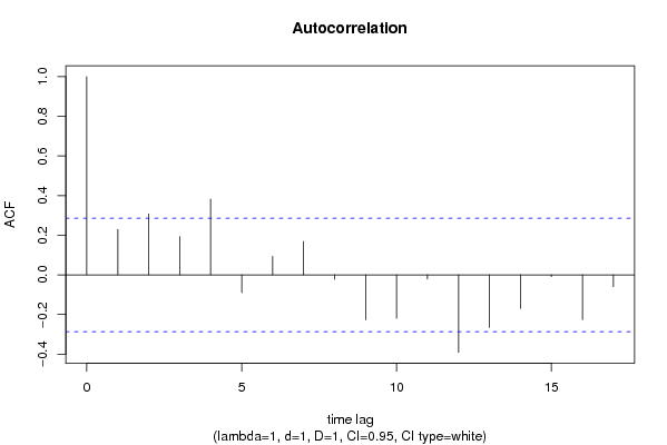
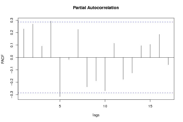
Title produced by software

(Partial) Autocorrelation Function

Date of computation

Fri, 27 Nov 2009 13:29:59 -0700

Cite this page as follows

Statistical Computations at FreeStatistics.org, Office for Research Development and Education, URL https://freestatistics.org/blog/index.php?v=date/2009/Nov/27/t1259353922kjj9nlrpaol14ho.htm/, Retrieved Sun, 28 Apr 2024 19:59:12 +0000

Statistical Computations at FreeStatistics.org, Office for Research Development and Education, URL https://freestatistics.org/blog/index.php?pk=61260, Retrieved Sun, 28 Apr 2024 19:59:12 +0000

QR Codes:

Paste this QR Code to cite your computation.

Original text written by user:

IsPrivate?

No (this computation is public)

User-defined keywords

Estimated Impact

199

Family? (F = Feedback message, R = changed R code, M = changed R Module, P = changed Parameters, D = changed Data)

-     [Univariate Explorative Data Analysis] [Run Sequence gebo...] [2008-12-12 13:32:37] [76963dc1903f0f612b6153510a3818cf]
- R  D  [Univariate Explorative Data Analysis] [Run Sequence gebo...] [2008-12-17 12:14:40] [76963dc1903f0f612b6153510a3818cf]
-         [Univariate Explorative Data Analysis] [Run Sequence Plot...] [2008-12-22 18:19:51] [1ce0d16c8f4225c977b42c8fa93bc163]
- RMP       [(Partial) Autocorrelation Function] [Identifying Integ...] [2009-11-22 12:16:10] [b98453cac15ba1066b407e146608df68]
-    D        [(Partial) Autocorrelation Function] [Model 1 (d = 0, D...] [2009-11-24 17:27:24] [ee7c2e7343f5b1451e62c5c16ec521f1]
-    D          [(Partial) Autocorrelation Function] [Methode 1 (D=0, d=0)] [2009-11-27 12:01:23] [76ab39dc7a55316678260825bd5ad46c]
-   P             [(Partial) Autocorrelation Function] [Methode 1 (d=1, D=0)] [2009-11-27 16:13:28] [76ab39dc7a55316678260825bd5ad46c]
-   P               [(Partial) Autocorrelation Function] [Methode 1 (d=1,D=1)] [2009-11-27 16:26:44] [76ab39dc7a55316678260825bd5ad46c]
-    D                  [(Partial) Autocorrelation Function] [methode 1 ( d=1 D...] [2009-11-27 20:29:59] [986e3c28a4248c495afaef9fd432264f] [Current]

Feedback Forum

Post a new message

Dataseries X:

Download CSV

Histogram

Boxplots

Summary of computational transaction
Raw Input	view raw input (R code)
Raw Output	view raw output of R engine
Computing time	1 seconds
R Server	'Gwilym Jenkins' @ 72.249.127.135

\begin{tabular}{lllllllll}
\hline
Summary of computational transaction \tabularnewline
Raw Input & view raw input (R code)  \tabularnewline
Raw Output & view raw output of R engine  \tabularnewline
Computing time & 1 seconds \tabularnewline
R Server & 'Gwilym Jenkins' @ 72.249.127.135 \tabularnewline
\hline
\end{tabular}
%Source: https://freestatistics.org/blog/index.php?pk=61260&T=0

[TABLE]
[ROW][C]Summary of computational transaction[/C][/ROW]
[ROW][C]Raw Input[/C][C]view raw input (R code) [/C][/ROW]
[ROW][C]Raw Output[/C][C]view raw output of R engine [/C][/ROW]
[ROW][C]Computing time[/C][C]1 seconds[/C][/ROW]
[ROW][C]R Server[/C][C]'Gwilym Jenkins' @ 72.249.127.135[/C][/ROW]
[/TABLE]
Source: https://freestatistics.org/blog/index.php?pk=61260&T=0

Globally Unique Identifier (entire table): ba.freestatistics.org/blog/index.php?pk=61260&T=0

As an alternative you can also use a QR Code:

The GUIDs for individual cells are displayed in the table below:

Summary of computational transaction
Raw Input	view raw input (R code)
Raw Output	view raw output of R engine
Computing time	1 seconds
R Server	'Gwilym Jenkins' @ 72.249.127.135

Autocorrelation Function
Time lag k	ACF(k)	T-STAT	P-value
1	0.229848	1.5758	0.060895
2	0.308077	2.1121	0.020012
3	0.19346	1.3263	0.095575
4	0.382561	2.6227	0.005861
5	-0.089325	-0.6124	0.271618
6	0.093331	0.6398	0.26269
7	0.168769	1.157	0.126555
8	-0.022102	-0.1515	0.440105
9	-0.226237	-1.551	0.063805
10	-0.218918	-1.5008	0.070045
11	-0.020583	-0.1411	0.444193
12	-0.390374	-2.6763	0.005108
13	-0.265301	-1.8188	0.037658
14	-0.169709	-1.1635	0.125256
15	-0.008792	-0.0603	0.476095
16	-0.225904	-1.5487	0.064078
17	-0.059142	-0.4055	0.34349

\begin{tabular}{lllllllll}
\hline
Autocorrelation Function \tabularnewline
Time lag k & ACF(k) & T-STAT & P-value \tabularnewline
1 & 0.229848 & 1.5758 & 0.060895 \tabularnewline
2 & 0.308077 & 2.1121 & 0.020012 \tabularnewline
3 & 0.19346 & 1.3263 & 0.095575 \tabularnewline
4 & 0.382561 & 2.6227 & 0.005861 \tabularnewline
5 & -0.089325 & -0.6124 & 0.271618 \tabularnewline
6 & 0.093331 & 0.6398 & 0.26269 \tabularnewline
7 & 0.168769 & 1.157 & 0.126555 \tabularnewline
8 & -0.022102 & -0.1515 & 0.440105 \tabularnewline
9 & -0.226237 & -1.551 & 0.063805 \tabularnewline
10 & -0.218918 & -1.5008 & 0.070045 \tabularnewline
11 & -0.020583 & -0.1411 & 0.444193 \tabularnewline
12 & -0.390374 & -2.6763 & 0.005108 \tabularnewline
13 & -0.265301 & -1.8188 & 0.037658 \tabularnewline
14 & -0.169709 & -1.1635 & 0.125256 \tabularnewline
15 & -0.008792 & -0.0603 & 0.476095 \tabularnewline
16 & -0.225904 & -1.5487 & 0.064078 \tabularnewline
17 & -0.059142 & -0.4055 & 0.34349 \tabularnewline
\hline
\end{tabular}
%Source: https://freestatistics.org/blog/index.php?pk=61260&T=1

[TABLE]
[ROW][C]Autocorrelation Function[/C][/ROW]
[ROW][C]Time lag k[/C][C]ACF(k)[/C][C]T-STAT[/C][C]P-value[/C][/ROW]
[ROW][C]1[/C][C]0.229848[/C][C]1.5758[/C][C]0.060895[/C][/ROW]
[ROW][C]2[/C][C]0.308077[/C][C]2.1121[/C][C]0.020012[/C][/ROW]
[ROW][C]3[/C][C]0.19346[/C][C]1.3263[/C][C]0.095575[/C][/ROW]
[ROW][C]4[/C][C]0.382561[/C][C]2.6227[/C][C]0.005861[/C][/ROW]
[ROW][C]5[/C][C]-0.089325[/C][C]-0.6124[/C][C]0.271618[/C][/ROW]
[ROW][C]6[/C][C]0.093331[/C][C]0.6398[/C][C]0.26269[/C][/ROW]
[ROW][C]7[/C][C]0.168769[/C][C]1.157[/C][C]0.126555[/C][/ROW]
[ROW][C]8[/C][C]-0.022102[/C][C]-0.1515[/C][C]0.440105[/C][/ROW]
[ROW][C]9[/C][C]-0.226237[/C][C]-1.551[/C][C]0.063805[/C][/ROW]
[ROW][C]10[/C][C]-0.218918[/C][C]-1.5008[/C][C]0.070045[/C][/ROW]
[ROW][C]11[/C][C]-0.020583[/C][C]-0.1411[/C][C]0.444193[/C][/ROW]
[ROW][C]12[/C][C]-0.390374[/C][C]-2.6763[/C][C]0.005108[/C][/ROW]
[ROW][C]13[/C][C]-0.265301[/C][C]-1.8188[/C][C]0.037658[/C][/ROW]
[ROW][C]14[/C][C]-0.169709[/C][C]-1.1635[/C][C]0.125256[/C][/ROW]
[ROW][C]15[/C][C]-0.008792[/C][C]-0.0603[/C][C]0.476095[/C][/ROW]
[ROW][C]16[/C][C]-0.225904[/C][C]-1.5487[/C][C]0.064078[/C][/ROW]
[ROW][C]17[/C][C]-0.059142[/C][C]-0.4055[/C][C]0.34349[/C][/ROW]
[/TABLE]
Source: https://freestatistics.org/blog/index.php?pk=61260&T=1

Globally Unique Identifier (entire table): ba.freestatistics.org/blog/index.php?pk=61260&T=1

As an alternative you can also use a QR Code:

The GUIDs for individual cells are displayed in the table below:

Autocorrelation Function
Time lag k	ACF(k)	T-STAT	P-value
1	0.229848	1.5758	0.060895
2	0.308077	2.1121	0.020012
3	0.19346	1.3263	0.095575
4	0.382561	2.6227	0.005861
5	-0.089325	-0.6124	0.271618
6	0.093331	0.6398	0.26269
7	0.168769	1.157	0.126555
8	-0.022102	-0.1515	0.440105
9	-0.226237	-1.551	0.063805
10	-0.218918	-1.5008	0.070045
11	-0.020583	-0.1411	0.444193
12	-0.390374	-2.6763	0.005108
13	-0.265301	-1.8188	0.037658
14	-0.169709	-1.1635	0.125256
15	-0.008792	-0.0603	0.476095
16	-0.225904	-1.5487	0.064078
17	-0.059142	-0.4055	0.34349

Partial Autocorrelation Function
Time lag k	PACF(k)	T-STAT	P-value
1	0.229848	1.5758	0.060895
2	0.269484	1.8475	0.035488
3	0.090839	0.6228	0.268226
4	0.293423	2.0116	0.025007
5	-0.315541	-2.1632	0.01782
6	-0.01701	-0.1166	0.453831
7	0.226214	1.5508	0.063824
8	-0.237348	-1.6272	0.055193
9	-0.189032	-1.2959	0.100662
10	-0.269046	-1.8445	0.03571
11	0.113869	0.7806	0.219462
12	-0.177143	-1.2144	0.115325
13	-0.125881	-0.863	0.19626
14	0.095018	0.6514	0.258976
15	0.105348	0.7222	0.236865
16	0.186069	1.2756	0.104178
17	-0.058932	-0.404	0.344017

\begin{tabular}{lllllllll}
\hline
Partial Autocorrelation Function \tabularnewline
Time lag k & PACF(k) & T-STAT & P-value \tabularnewline
1 & 0.229848 & 1.5758 & 0.060895 \tabularnewline
2 & 0.269484 & 1.8475 & 0.035488 \tabularnewline
3 & 0.090839 & 0.6228 & 0.268226 \tabularnewline
4 & 0.293423 & 2.0116 & 0.025007 \tabularnewline
5 & -0.315541 & -2.1632 & 0.01782 \tabularnewline
6 & -0.01701 & -0.1166 & 0.453831 \tabularnewline
7 & 0.226214 & 1.5508 & 0.063824 \tabularnewline
8 & -0.237348 & -1.6272 & 0.055193 \tabularnewline
9 & -0.189032 & -1.2959 & 0.100662 \tabularnewline
10 & -0.269046 & -1.8445 & 0.03571 \tabularnewline
11 & 0.113869 & 0.7806 & 0.219462 \tabularnewline
12 & -0.177143 & -1.2144 & 0.115325 \tabularnewline
13 & -0.125881 & -0.863 & 0.19626 \tabularnewline
14 & 0.095018 & 0.6514 & 0.258976 \tabularnewline
15 & 0.105348 & 0.7222 & 0.236865 \tabularnewline
16 & 0.186069 & 1.2756 & 0.104178 \tabularnewline
17 & -0.058932 & -0.404 & 0.344017 \tabularnewline
\hline
\end{tabular}
%Source: https://freestatistics.org/blog/index.php?pk=61260&T=2

[TABLE]
[ROW][C]Partial Autocorrelation Function[/C][/ROW]
[ROW][C]Time lag k[/C][C]PACF(k)[/C][C]T-STAT[/C][C]P-value[/C][/ROW]
[ROW][C]1[/C][C]0.229848[/C][C]1.5758[/C][C]0.060895[/C][/ROW]
[ROW][C]2[/C][C]0.269484[/C][C]1.8475[/C][C]0.035488[/C][/ROW]
[ROW][C]3[/C][C]0.090839[/C][C]0.6228[/C][C]0.268226[/C][/ROW]
[ROW][C]4[/C][C]0.293423[/C][C]2.0116[/C][C]0.025007[/C][/ROW]
[ROW][C]5[/C][C]-0.315541[/C][C]-2.1632[/C][C]0.01782[/C][/ROW]
[ROW][C]6[/C][C]-0.01701[/C][C]-0.1166[/C][C]0.453831[/C][/ROW]
[ROW][C]7[/C][C]0.226214[/C][C]1.5508[/C][C]0.063824[/C][/ROW]
[ROW][C]8[/C][C]-0.237348[/C][C]-1.6272[/C][C]0.055193[/C][/ROW]
[ROW][C]9[/C][C]-0.189032[/C][C]-1.2959[/C][C]0.100662[/C][/ROW]
[ROW][C]10[/C][C]-0.269046[/C][C]-1.8445[/C][C]0.03571[/C][/ROW]
[ROW][C]11[/C][C]0.113869[/C][C]0.7806[/C][C]0.219462[/C][/ROW]
[ROW][C]12[/C][C]-0.177143[/C][C]-1.2144[/C][C]0.115325[/C][/ROW]
[ROW][C]13[/C][C]-0.125881[/C][C]-0.863[/C][C]0.19626[/C][/ROW]
[ROW][C]14[/C][C]0.095018[/C][C]0.6514[/C][C]0.258976[/C][/ROW]
[ROW][C]15[/C][C]0.105348[/C][C]0.7222[/C][C]0.236865[/C][/ROW]
[ROW][C]16[/C][C]0.186069[/C][C]1.2756[/C][C]0.104178[/C][/ROW]
[ROW][C]17[/C][C]-0.058932[/C][C]-0.404[/C][C]0.344017[/C][/ROW]
[/TABLE]
Source: https://freestatistics.org/blog/index.php?pk=61260&T=2

Globally Unique Identifier (entire table): ba.freestatistics.org/blog/index.php?pk=61260&T=2

As an alternative you can also use a QR Code:

The GUIDs for individual cells are displayed in the table below:

Partial Autocorrelation Function
Time lag k	PACF(k)	T-STAT	P-value
1	0.229848	1.5758	0.060895
2	0.269484	1.8475	0.035488
3	0.090839	0.6228	0.268226
4	0.293423	2.0116	0.025007
5	-0.315541	-2.1632	0.01782
6	-0.01701	-0.1166	0.453831
7	0.226214	1.5508	0.063824
8	-0.237348	-1.6272	0.055193
9	-0.189032	-1.2959	0.100662
10	-0.269046	-1.8445	0.03571
11	0.113869	0.7806	0.219462
12	-0.177143	-1.2144	0.115325
13	-0.125881	-0.863	0.19626
14	0.095018	0.6514	0.258976
15	0.105348	0.7222	0.236865
16	0.186069	1.2756	0.104178
17	-0.058932	-0.404	0.344017

Figure 1

PNG link

Postscript link

PDF link

Figure 2

PNG link

Postscript link

PDF link

Parameters (Session):

par1 = Default ; par2 = 1 ; par3 = 1 ; par4 = 1 ; par5 = 12 ; par6 = White Noise ; par7 = 0.95 ;

Parameters (R input):

par1 = Default ; par2 = 1 ; par3 = 1 ; par4 = 1 ; par5 = 12 ; par6 = White Noise ; par7 = 0.95 ;

R code (references can be found in the software module):

if (par1 == 'Default') {
par1 = 10*log10(length(x))
} else {
par1 <- as.numeric(par1)
}
par2 <- as.numeric(par2)
par3 <- as.numeric(par3)
par4 <- as.numeric(par4)
par5 <- as.numeric(par5)
if (par6 == 'White Noise') par6 <- 'white' else par6 <- 'ma'
par7 <- as.numeric(par7)
if (par2 == 0) {
x <- log(x)
} else {
x <- (x ^ par2 - 1) / par2
}
if (par3 > 0) x <- diff(x,lag=1,difference=par3)
if (par4 > 0) x <- diff(x,lag=par5,difference=par4)
bitmap(file='pic1.png')
racf <- acf(x, par1, main='Autocorrelation', xlab='time lag', ylab='ACF', ci.type=par6, ci=par7, sub=paste('(lambda=',par2,', d=',par3,', D=',par4,', CI=', par7, ', CI type=',par6,')',sep=''))
dev.off()
bitmap(file='pic2.png')
rpacf <- pacf(x,par1,main='Partial Autocorrelation',xlab='lags',ylab='PACF')
dev.off()
(myacf <- c(racf$acf))
(mypacf <- c(rpacf$acf))
lengthx <- length(x)
sqrtn <- sqrt(lengthx)
load(file='createtable')
a<-table.start()
a<-table.row.start(a)
a<-table.element(a,'Autocorrelation Function',4,TRUE)
a<-table.row.end(a)
a<-table.row.start(a)
a<-table.element(a,'Time lag k',header=TRUE)
a<-table.element(a,hyperlink('basics.htm','ACF(k)','click here for more information about the Autocorrelation Function'),header=TRUE)
a<-table.element(a,'T-STAT',header=TRUE)
a<-table.element(a,'P-value',header=TRUE)
a<-table.row.end(a)
for (i in 2:(par1+1)) {
a<-table.row.start(a)
a<-table.element(a,i-1,header=TRUE)
a<-table.element(a,round(myacf[i],6))
mytstat <- myacf[i]*sqrtn
a<-table.element(a,round(mytstat,4))
a<-table.element(a,round(1-pt(abs(mytstat),lengthx),6))
a<-table.row.end(a)
}
a<-table.end(a)
table.save(a,file='mytable.tab')
a<-table.start()
a<-table.row.start(a)
a<-table.element(a,'Partial Autocorrelation Function',4,TRUE)
a<-table.row.end(a)
a<-table.row.start(a)
a<-table.element(a,'Time lag k',header=TRUE)
a<-table.element(a,hyperlink('basics.htm','PACF(k)','click here for more information about the Partial Autocorrelation Function'),header=TRUE)
a<-table.element(a,'T-STAT',header=TRUE)
a<-table.element(a,'P-value',header=TRUE)
a<-table.row.end(a)
for (i in 1:par1) {
a<-table.row.start(a)
a<-table.element(a,i,header=TRUE)
a<-table.element(a,round(mypacf[i],6))
mytstat <- mypacf[i]*sqrtn
a<-table.element(a,round(mytstat,4))
a<-table.element(a,round(1-pt(abs(mytstat),lengthx),6))
a<-table.row.end(a)
}
a<-table.end(a)
table.save(a,file='mytable1.tab')

Free Statistics

Description of Statistical Computation

Tree of Dependent Computations

Dataset

Tables (Output of Computation)

Figures (Output of Computation)

Input Parameters & R Code