Repository of Reproducible Computations

Free Statistics

of Irreproducible Research!

Author's title

Author

*The author of this computation has been verified*

R Software Module

rwasp_autocorrelation.wasp

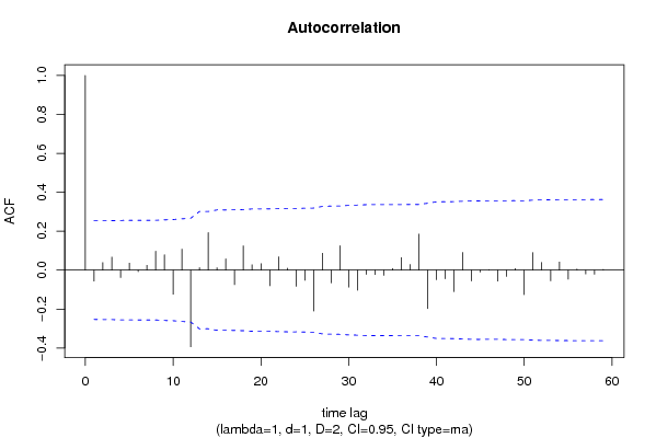
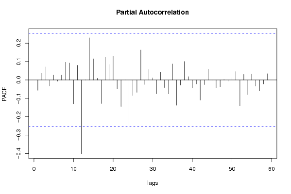
Title produced by software

(Partial) Autocorrelation Function

Date of computation

Fri, 27 Nov 2009 13:58:47 -0700

Cite this page as follows

Statistical Computations at FreeStatistics.org, Office for Research Development and Education, URL https://freestatistics.org/blog/index.php?v=date/2009/Nov/27/t125935562644glid621ab4vte.htm/, Retrieved Sun, 28 Apr 2024 20:51:54 +0000

Statistical Computations at FreeStatistics.org, Office for Research Development and Education, URL https://freestatistics.org/blog/index.php?pk=61277, Retrieved Sun, 28 Apr 2024 20:51:54 +0000

QR Codes:

Paste this QR Code to cite your computation.

Original text written by user:

IsPrivate?

No (this computation is public)

User-defined keywords

Estimated Impact

146

Family? (F = Feedback message, R = changed R code, M = changed R Module, P = changed Parameters, D = changed Data)

-     [Univariate Explorative Data Analysis] [Run Sequence gebo...] [2008-12-12 13:32:37] [76963dc1903f0f612b6153510a3818cf]
- R  D  [Univariate Explorative Data Analysis] [Run Sequence gebo...] [2008-12-17 12:14:40] [76963dc1903f0f612b6153510a3818cf]
-         [Univariate Explorative Data Analysis] [Run Sequence Plot...] [2008-12-22 18:19:51] [1ce0d16c8f4225c977b42c8fa93bc163]
- RMP       [(Partial) Autocorrelation Function] [Identifying Integ...] [2009-11-22 12:16:10] [b98453cac15ba1066b407e146608df68]
-   PD        [(Partial) Autocorrelation Function] [Workshop 8] [2009-11-24 11:49:44] [214e6e00abbde49700521a7ef1d30da2]
-    D          [(Partial) Autocorrelation Function] [WS 8.2 autocorrel...] [2009-11-27 20:13:42] [d31db4f83c6a129f6d3e47077769e868]
-   P               [(Partial) Autocorrelation Function] [WS 8.4 Autocorrel...] [2009-11-27 20:58:47] [852eae237d08746109043531619a60c9] [Current]
- RM                  [Variance Reduction Matrix] [WS 8.5 Variantie ...] [2009-11-27 21:11:14] [d31db4f83c6a129f6d3e47077769e868] 
- RM                    [Spectral Analysis] [WS 8.7 Spectrum a...] [2009-11-27 21:40:54] [d31db4f83c6a129f6d3e47077769e868] 
-                         [Spectral Analysis] [WS 8.8 Spectrum a...] [2009-11-27 21:57:05] [d31db4f83c6a129f6d3e47077769e868] 
- RM                        [Standard Deviation-Mean Plot] [WS 8.9 Heterosked...] [2009-11-27 22:13:36] [d31db4f83c6a129f6d3e47077769e868] 
-   P                 [(Partial) Autocorrelation Function] [SHWWS8review2] [2009-11-29 14:37:49] [a66d3a79ef9e5308cd94a469bc5ca464] 

Feedback Forum

Post a new message

Dataseries X:

Download CSV

Histogram

Boxplots

Summary of computational transaction
Raw Input	view raw input (R code)
Raw Output	view raw output of R engine
Computing time	1 seconds
R Server	'Gwilym Jenkins' @ 72.249.127.135

\begin{tabular}{lllllllll}
\hline
Summary of computational transaction \tabularnewline
Raw Input & view raw input (R code)  \tabularnewline
Raw Output & view raw output of R engine  \tabularnewline
Computing time & 1 seconds \tabularnewline
R Server & 'Gwilym Jenkins' @ 72.249.127.135 \tabularnewline
\hline
\end{tabular}
%Source: https://freestatistics.org/blog/index.php?pk=61277&T=0

[TABLE]
[ROW][C]Summary of computational transaction[/C][/ROW]
[ROW][C]Raw Input[/C][C]view raw input (R code) [/C][/ROW]
[ROW][C]Raw Output[/C][C]view raw output of R engine [/C][/ROW]
[ROW][C]Computing time[/C][C]1 seconds[/C][/ROW]
[ROW][C]R Server[/C][C]'Gwilym Jenkins' @ 72.249.127.135[/C][/ROW]
[/TABLE]
Source: https://freestatistics.org/blog/index.php?pk=61277&T=0

Globally Unique Identifier (entire table): ba.freestatistics.org/blog/index.php?pk=61277&T=0

As an alternative you can also use a QR Code:

The GUIDs for individual cells are displayed in the table below:

Summary of computational transaction
Raw Input	view raw input (R code)
Raw Output	view raw output of R engine
Computing time	1 seconds
R Server	'Gwilym Jenkins' @ 72.249.127.135

Autocorrelation Function
Time lag k	ACF(k)	T-STAT	P-value
1	-0.056255	-0.4358	0.33229
2	0.039139	0.3032	0.381404
3	0.066607	0.5159	0.303898
4	-0.037932	-0.2938	0.384953
5	0.035971	0.2786	0.390744
6	-0.007798	-0.0604	0.476017
7	0.024951	0.1933	0.423699
8	0.097435	0.7547	0.226683
9	0.078635	0.6091	0.272377
10	-0.123864	-0.9594	0.170592
11	0.107856	0.8354	0.20339
12	-0.393497	-3.048	0.001712
13	0.012556	0.0973	0.461423
14	0.192704	1.4927	0.070381
15	0.01198	0.0928	0.463186
16	0.058048	0.4496	0.327297
17	-0.074491	-0.577	0.283048
18	0.124571	0.9649	0.169228
19	0.027213	0.2108	0.416881
20	0.032921	0.255	0.399796
21	-0.080248	-0.6216	0.268281
22	0.068218	0.5284	0.299581
23	0.009827	0.0761	0.469788
24	-0.083057	-0.6434	0.261221
25	-0.05167	-0.4002	0.345203
26	-0.210452	-1.6302	0.054154
27	0.086365	0.669	0.253037
28	-0.06505	-0.5039	0.308097
29	0.125003	0.9683	0.168398
30	-0.086781	-0.6722	0.252017
31	-0.103121	-0.7988	0.213787
32	-0.021666	-0.1678	0.433644
33	-0.022683	-0.1757	0.430561
34	-0.026337	-0.204	0.419521
35	0.008307	0.0643	0.474455
36	0.063972	0.4955	0.31102
37	0.029044	0.225	0.411382
38	0.184711	1.4308	0.078843
39	-0.197687	-1.5313	0.065478
40	-0.049365	-0.3824	0.351765
41	-0.044358	-0.3436	0.366175
42	-0.110636	-0.857	0.197432
43	0.090515	0.7011	0.242966
44	-0.055695	-0.4314	0.333859
45	-0.009718	-0.0753	0.470122
46	0.002146	0.0166	0.493395
47	-0.055819	-0.4324	0.333511
48	-0.032066	-0.2484	0.402343
49	0.007509	0.0582	0.476906
50	-0.125715	-0.9738	0.167037
51	0.089946	0.6967	0.244336
52	0.039736	0.3078	0.379654
53	-0.054415	-0.4215	0.337448
54	0.041453	0.3211	0.374627
55	-0.046564	-0.3607	0.359802
56	0.006068	0.047	0.481335
57	-0.0195	-0.151	0.440222
58	-0.020946	-0.1622	0.435829
59	0.003979	0.0308	0.487758
60	NA	NA	NA

\begin{tabular}{lllllllll}
\hline
Autocorrelation Function \tabularnewline
Time lag k & ACF(k) & T-STAT & P-value \tabularnewline
1 & -0.056255 & -0.4358 & 0.33229 \tabularnewline
2 & 0.039139 & 0.3032 & 0.381404 \tabularnewline
3 & 0.066607 & 0.5159 & 0.303898 \tabularnewline
4 & -0.037932 & -0.2938 & 0.384953 \tabularnewline
5 & 0.035971 & 0.2786 & 0.390744 \tabularnewline
6 & -0.007798 & -0.0604 & 0.476017 \tabularnewline
7 & 0.024951 & 0.1933 & 0.423699 \tabularnewline
8 & 0.097435 & 0.7547 & 0.226683 \tabularnewline
9 & 0.078635 & 0.6091 & 0.272377 \tabularnewline
10 & -0.123864 & -0.9594 & 0.170592 \tabularnewline
11 & 0.107856 & 0.8354 & 0.20339 \tabularnewline
12 & -0.393497 & -3.048 & 0.001712 \tabularnewline
13 & 0.012556 & 0.0973 & 0.461423 \tabularnewline
14 & 0.192704 & 1.4927 & 0.070381 \tabularnewline
15 & 0.01198 & 0.0928 & 0.463186 \tabularnewline
16 & 0.058048 & 0.4496 & 0.327297 \tabularnewline
17 & -0.074491 & -0.577 & 0.283048 \tabularnewline
18 & 0.124571 & 0.9649 & 0.169228 \tabularnewline
19 & 0.027213 & 0.2108 & 0.416881 \tabularnewline
20 & 0.032921 & 0.255 & 0.399796 \tabularnewline
21 & -0.080248 & -0.6216 & 0.268281 \tabularnewline
22 & 0.068218 & 0.5284 & 0.299581 \tabularnewline
23 & 0.009827 & 0.0761 & 0.469788 \tabularnewline
24 & -0.083057 & -0.6434 & 0.261221 \tabularnewline
25 & -0.05167 & -0.4002 & 0.345203 \tabularnewline
26 & -0.210452 & -1.6302 & 0.054154 \tabularnewline
27 & 0.086365 & 0.669 & 0.253037 \tabularnewline
28 & -0.06505 & -0.5039 & 0.308097 \tabularnewline
29 & 0.125003 & 0.9683 & 0.168398 \tabularnewline
30 & -0.086781 & -0.6722 & 0.252017 \tabularnewline
31 & -0.103121 & -0.7988 & 0.213787 \tabularnewline
32 & -0.021666 & -0.1678 & 0.433644 \tabularnewline
33 & -0.022683 & -0.1757 & 0.430561 \tabularnewline
34 & -0.026337 & -0.204 & 0.419521 \tabularnewline
35 & 0.008307 & 0.0643 & 0.474455 \tabularnewline
36 & 0.063972 & 0.4955 & 0.31102 \tabularnewline
37 & 0.029044 & 0.225 & 0.411382 \tabularnewline
38 & 0.184711 & 1.4308 & 0.078843 \tabularnewline
39 & -0.197687 & -1.5313 & 0.065478 \tabularnewline
40 & -0.049365 & -0.3824 & 0.351765 \tabularnewline
41 & -0.044358 & -0.3436 & 0.366175 \tabularnewline
42 & -0.110636 & -0.857 & 0.197432 \tabularnewline
43 & 0.090515 & 0.7011 & 0.242966 \tabularnewline
44 & -0.055695 & -0.4314 & 0.333859 \tabularnewline
45 & -0.009718 & -0.0753 & 0.470122 \tabularnewline
46 & 0.002146 & 0.0166 & 0.493395 \tabularnewline
47 & -0.055819 & -0.4324 & 0.333511 \tabularnewline
48 & -0.032066 & -0.2484 & 0.402343 \tabularnewline
49 & 0.007509 & 0.0582 & 0.476906 \tabularnewline
50 & -0.125715 & -0.9738 & 0.167037 \tabularnewline
51 & 0.089946 & 0.6967 & 0.244336 \tabularnewline
52 & 0.039736 & 0.3078 & 0.379654 \tabularnewline
53 & -0.054415 & -0.4215 & 0.337448 \tabularnewline
54 & 0.041453 & 0.3211 & 0.374627 \tabularnewline
55 & -0.046564 & -0.3607 & 0.359802 \tabularnewline
56 & 0.006068 & 0.047 & 0.481335 \tabularnewline
57 & -0.0195 & -0.151 & 0.440222 \tabularnewline
58 & -0.020946 & -0.1622 & 0.435829 \tabularnewline
59 & 0.003979 & 0.0308 & 0.487758 \tabularnewline
60 & NA & NA & NA \tabularnewline
\hline
\end{tabular}
%Source: https://freestatistics.org/blog/index.php?pk=61277&T=1

[TABLE]
[ROW][C]Autocorrelation Function[/C][/ROW]
[ROW][C]Time lag k[/C][C]ACF(k)[/C][C]T-STAT[/C][C]P-value[/C][/ROW]
[ROW][C]1[/C][C]-0.056255[/C][C]-0.4358[/C][C]0.33229[/C][/ROW]
[ROW][C]2[/C][C]0.039139[/C][C]0.3032[/C][C]0.381404[/C][/ROW]
[ROW][C]3[/C][C]0.066607[/C][C]0.5159[/C][C]0.303898[/C][/ROW]
[ROW][C]4[/C][C]-0.037932[/C][C]-0.2938[/C][C]0.384953[/C][/ROW]
[ROW][C]5[/C][C]0.035971[/C][C]0.2786[/C][C]0.390744[/C][/ROW]
[ROW][C]6[/C][C]-0.007798[/C][C]-0.0604[/C][C]0.476017[/C][/ROW]
[ROW][C]7[/C][C]0.024951[/C][C]0.1933[/C][C]0.423699[/C][/ROW]
[ROW][C]8[/C][C]0.097435[/C][C]0.7547[/C][C]0.226683[/C][/ROW]
[ROW][C]9[/C][C]0.078635[/C][C]0.6091[/C][C]0.272377[/C][/ROW]
[ROW][C]10[/C][C]-0.123864[/C][C]-0.9594[/C][C]0.170592[/C][/ROW]
[ROW][C]11[/C][C]0.107856[/C][C]0.8354[/C][C]0.20339[/C][/ROW]
[ROW][C]12[/C][C]-0.393497[/C][C]-3.048[/C][C]0.001712[/C][/ROW]
[ROW][C]13[/C][C]0.012556[/C][C]0.0973[/C][C]0.461423[/C][/ROW]
[ROW][C]14[/C][C]0.192704[/C][C]1.4927[/C][C]0.070381[/C][/ROW]
[ROW][C]15[/C][C]0.01198[/C][C]0.0928[/C][C]0.463186[/C][/ROW]
[ROW][C]16[/C][C]0.058048[/C][C]0.4496[/C][C]0.327297[/C][/ROW]
[ROW][C]17[/C][C]-0.074491[/C][C]-0.577[/C][C]0.283048[/C][/ROW]
[ROW][C]18[/C][C]0.124571[/C][C]0.9649[/C][C]0.169228[/C][/ROW]
[ROW][C]19[/C][C]0.027213[/C][C]0.2108[/C][C]0.416881[/C][/ROW]
[ROW][C]20[/C][C]0.032921[/C][C]0.255[/C][C]0.399796[/C][/ROW]
[ROW][C]21[/C][C]-0.080248[/C][C]-0.6216[/C][C]0.268281[/C][/ROW]
[ROW][C]22[/C][C]0.068218[/C][C]0.5284[/C][C]0.299581[/C][/ROW]
[ROW][C]23[/C][C]0.009827[/C][C]0.0761[/C][C]0.469788[/C][/ROW]
[ROW][C]24[/C][C]-0.083057[/C][C]-0.6434[/C][C]0.261221[/C][/ROW]
[ROW][C]25[/C][C]-0.05167[/C][C]-0.4002[/C][C]0.345203[/C][/ROW]
[ROW][C]26[/C][C]-0.210452[/C][C]-1.6302[/C][C]0.054154[/C][/ROW]
[ROW][C]27[/C][C]0.086365[/C][C]0.669[/C][C]0.253037[/C][/ROW]
[ROW][C]28[/C][C]-0.06505[/C][C]-0.5039[/C][C]0.308097[/C][/ROW]
[ROW][C]29[/C][C]0.125003[/C][C]0.9683[/C][C]0.168398[/C][/ROW]
[ROW][C]30[/C][C]-0.086781[/C][C]-0.6722[/C][C]0.252017[/C][/ROW]
[ROW][C]31[/C][C]-0.103121[/C][C]-0.7988[/C][C]0.213787[/C][/ROW]
[ROW][C]32[/C][C]-0.021666[/C][C]-0.1678[/C][C]0.433644[/C][/ROW]
[ROW][C]33[/C][C]-0.022683[/C][C]-0.1757[/C][C]0.430561[/C][/ROW]
[ROW][C]34[/C][C]-0.026337[/C][C]-0.204[/C][C]0.419521[/C][/ROW]
[ROW][C]35[/C][C]0.008307[/C][C]0.0643[/C][C]0.474455[/C][/ROW]
[ROW][C]36[/C][C]0.063972[/C][C]0.4955[/C][C]0.31102[/C][/ROW]
[ROW][C]37[/C][C]0.029044[/C][C]0.225[/C][C]0.411382[/C][/ROW]
[ROW][C]38[/C][C]0.184711[/C][C]1.4308[/C][C]0.078843[/C][/ROW]
[ROW][C]39[/C][C]-0.197687[/C][C]-1.5313[/C][C]0.065478[/C][/ROW]
[ROW][C]40[/C][C]-0.049365[/C][C]-0.3824[/C][C]0.351765[/C][/ROW]
[ROW][C]41[/C][C]-0.044358[/C][C]-0.3436[/C][C]0.366175[/C][/ROW]
[ROW][C]42[/C][C]-0.110636[/C][C]-0.857[/C][C]0.197432[/C][/ROW]
[ROW][C]43[/C][C]0.090515[/C][C]0.7011[/C][C]0.242966[/C][/ROW]
[ROW][C]44[/C][C]-0.055695[/C][C]-0.4314[/C][C]0.333859[/C][/ROW]
[ROW][C]45[/C][C]-0.009718[/C][C]-0.0753[/C][C]0.470122[/C][/ROW]
[ROW][C]46[/C][C]0.002146[/C][C]0.0166[/C][C]0.493395[/C][/ROW]
[ROW][C]47[/C][C]-0.055819[/C][C]-0.4324[/C][C]0.333511[/C][/ROW]
[ROW][C]48[/C][C]-0.032066[/C][C]-0.2484[/C][C]0.402343[/C][/ROW]
[ROW][C]49[/C][C]0.007509[/C][C]0.0582[/C][C]0.476906[/C][/ROW]
[ROW][C]50[/C][C]-0.125715[/C][C]-0.9738[/C][C]0.167037[/C][/ROW]
[ROW][C]51[/C][C]0.089946[/C][C]0.6967[/C][C]0.244336[/C][/ROW]
[ROW][C]52[/C][C]0.039736[/C][C]0.3078[/C][C]0.379654[/C][/ROW]
[ROW][C]53[/C][C]-0.054415[/C][C]-0.4215[/C][C]0.337448[/C][/ROW]
[ROW][C]54[/C][C]0.041453[/C][C]0.3211[/C][C]0.374627[/C][/ROW]
[ROW][C]55[/C][C]-0.046564[/C][C]-0.3607[/C][C]0.359802[/C][/ROW]
[ROW][C]56[/C][C]0.006068[/C][C]0.047[/C][C]0.481335[/C][/ROW]
[ROW][C]57[/C][C]-0.0195[/C][C]-0.151[/C][C]0.440222[/C][/ROW]
[ROW][C]58[/C][C]-0.020946[/C][C]-0.1622[/C][C]0.435829[/C][/ROW]
[ROW][C]59[/C][C]0.003979[/C][C]0.0308[/C][C]0.487758[/C][/ROW]
[ROW][C]60[/C][C]NA[/C][C]NA[/C][C]NA[/C][/ROW]
[/TABLE]
Source: https://freestatistics.org/blog/index.php?pk=61277&T=1

Globally Unique Identifier (entire table): ba.freestatistics.org/blog/index.php?pk=61277&T=1

As an alternative you can also use a QR Code:

The GUIDs for individual cells are displayed in the table below:

Autocorrelation Function
Time lag k	ACF(k)	T-STAT	P-value
1	-0.056255	-0.4358	0.33229
2	0.039139	0.3032	0.381404
3	0.066607	0.5159	0.303898
4	-0.037932	-0.2938	0.384953
5	0.035971	0.2786	0.390744
6	-0.007798	-0.0604	0.476017
7	0.024951	0.1933	0.423699
8	0.097435	0.7547	0.226683
9	0.078635	0.6091	0.272377
10	-0.123864	-0.9594	0.170592
11	0.107856	0.8354	0.20339
12	-0.393497	-3.048	0.001712
13	0.012556	0.0973	0.461423
14	0.192704	1.4927	0.070381
15	0.01198	0.0928	0.463186
16	0.058048	0.4496	0.327297
17	-0.074491	-0.577	0.283048
18	0.124571	0.9649	0.169228
19	0.027213	0.2108	0.416881
20	0.032921	0.255	0.399796
21	-0.080248	-0.6216	0.268281
22	0.068218	0.5284	0.299581
23	0.009827	0.0761	0.469788
24	-0.083057	-0.6434	0.261221
25	-0.05167	-0.4002	0.345203
26	-0.210452	-1.6302	0.054154
27	0.086365	0.669	0.253037
28	-0.06505	-0.5039	0.308097
29	0.125003	0.9683	0.168398
30	-0.086781	-0.6722	0.252017
31	-0.103121	-0.7988	0.213787
32	-0.021666	-0.1678	0.433644
33	-0.022683	-0.1757	0.430561
34	-0.026337	-0.204	0.419521
35	0.008307	0.0643	0.474455
36	0.063972	0.4955	0.31102
37	0.029044	0.225	0.411382
38	0.184711	1.4308	0.078843
39	-0.197687	-1.5313	0.065478
40	-0.049365	-0.3824	0.351765
41	-0.044358	-0.3436	0.366175
42	-0.110636	-0.857	0.197432
43	0.090515	0.7011	0.242966
44	-0.055695	-0.4314	0.333859
45	-0.009718	-0.0753	0.470122
46	0.002146	0.0166	0.493395
47	-0.055819	-0.4324	0.333511
48	-0.032066	-0.2484	0.402343
49	0.007509	0.0582	0.476906
50	-0.125715	-0.9738	0.167037
51	0.089946	0.6967	0.244336
52	0.039736	0.3078	0.379654
53	-0.054415	-0.4215	0.337448
54	0.041453	0.3211	0.374627
55	-0.046564	-0.3607	0.359802
56	0.006068	0.047	0.481335
57	-0.0195	-0.151	0.440222
58	-0.020946	-0.1622	0.435829
59	0.003979	0.0308	0.487758
60	NA	NA	NA

Partial Autocorrelation Function
Time lag k	PACF(k)	T-STAT	P-value
1	-0.056255	-0.4358	0.33229
2	0.036089	0.2795	0.390395
3	0.071077	0.5506	0.291991
4	-0.032019	-0.248	0.402485
5	0.026928	0.2086	0.417739
6	-0.006274	-0.0486	0.480699
7	0.026652	0.2064	0.418572
8	0.096492	0.7474	0.228862
9	0.092094	0.7134	0.239196
10	-0.130048	-1.0074	0.158906
11	0.079552	0.6162	0.270044
12	-0.400227	-3.1001	0.001472
13	0.001019	0.0079	0.496863
14	0.229441	1.7772	0.040298
15	0.115281	0.893	0.187723
16	0.009098	0.0705	0.472027
17	-0.127905	-0.9907	0.162894
18	0.12394	0.96	0.170445
19	0.084293	0.6529	0.258148
20	0.128604	0.9962	0.161586
21	-0.049481	-0.3833	0.351433
22	-0.144133	-1.1164	0.134341
23	0.001253	0.0097	0.496145
24	-0.247993	-1.9209	0.029747
25	-0.084744	-0.6564	0.25703
26	-0.067298	-0.5213	0.302041
27	0.163236	1.2644	0.105485
28	-0.024812	-0.1922	0.424121
29	0.056938	0.441	0.330385
30	0.011835	0.0917	0.463632
31	-0.075257	-0.5829	0.28106
32	0.042006	0.3254	0.373013
33	-0.041198	-0.3191	0.375373
34	-0.075894	-0.5879	0.279411
35	0.08734	0.6765	0.250651
36	-0.137703	-1.0666	0.145203
37	-0.027837	-0.2156	0.415006
38	0.100468	0.7782	0.219749
39	0.018458	0.143	0.443395
40	-0.043169	-0.3344	0.369628
41	-0.021402	-0.1658	0.434445
42	-0.109417	-0.8475	0.200031
43	-0.025119	-0.1946	0.423194
44	0.058953	0.4567	0.324786
45	-0.001357	-0.0105	0.495825
46	-0.042323	-0.3278	0.372091
47	-0.036409	-0.282	0.389449
48	0.002244	0.0174	0.493094
49	-0.006108	-0.0473	0.481212
50	0.012617	0.0977	0.461234
51	0.045842	0.3551	0.361885
52	-0.141403	-1.0953	0.138881
53	0.030152	0.2336	0.408062
54	-0.079793	-0.6181	0.269432
55	0.032663	0.253	0.400565
56	-0.033289	-0.2579	0.3987
57	-0.059534	-0.4611	0.32318
58	-0.021656	-0.1677	0.433674
59	0.034311	0.2658	0.395664
60	NA	NA	NA

\begin{tabular}{lllllllll}
\hline
Partial Autocorrelation Function \tabularnewline
Time lag k & PACF(k) & T-STAT & P-value \tabularnewline
1 & -0.056255 & -0.4358 & 0.33229 \tabularnewline
2 & 0.036089 & 0.2795 & 0.390395 \tabularnewline
3 & 0.071077 & 0.5506 & 0.291991 \tabularnewline
4 & -0.032019 & -0.248 & 0.402485 \tabularnewline
5 & 0.026928 & 0.2086 & 0.417739 \tabularnewline
6 & -0.006274 & -0.0486 & 0.480699 \tabularnewline
7 & 0.026652 & 0.2064 & 0.418572 \tabularnewline
8 & 0.096492 & 0.7474 & 0.228862 \tabularnewline
9 & 0.092094 & 0.7134 & 0.239196 \tabularnewline
10 & -0.130048 & -1.0074 & 0.158906 \tabularnewline
11 & 0.079552 & 0.6162 & 0.270044 \tabularnewline
12 & -0.400227 & -3.1001 & 0.001472 \tabularnewline
13 & 0.001019 & 0.0079 & 0.496863 \tabularnewline
14 & 0.229441 & 1.7772 & 0.040298 \tabularnewline
15 & 0.115281 & 0.893 & 0.187723 \tabularnewline
16 & 0.009098 & 0.0705 & 0.472027 \tabularnewline
17 & -0.127905 & -0.9907 & 0.162894 \tabularnewline
18 & 0.12394 & 0.96 & 0.170445 \tabularnewline
19 & 0.084293 & 0.6529 & 0.258148 \tabularnewline
20 & 0.128604 & 0.9962 & 0.161586 \tabularnewline
21 & -0.049481 & -0.3833 & 0.351433 \tabularnewline
22 & -0.144133 & -1.1164 & 0.134341 \tabularnewline
23 & 0.001253 & 0.0097 & 0.496145 \tabularnewline
24 & -0.247993 & -1.9209 & 0.029747 \tabularnewline
25 & -0.084744 & -0.6564 & 0.25703 \tabularnewline
26 & -0.067298 & -0.5213 & 0.302041 \tabularnewline
27 & 0.163236 & 1.2644 & 0.105485 \tabularnewline
28 & -0.024812 & -0.1922 & 0.424121 \tabularnewline
29 & 0.056938 & 0.441 & 0.330385 \tabularnewline
30 & 0.011835 & 0.0917 & 0.463632 \tabularnewline
31 & -0.075257 & -0.5829 & 0.28106 \tabularnewline
32 & 0.042006 & 0.3254 & 0.373013 \tabularnewline
33 & -0.041198 & -0.3191 & 0.375373 \tabularnewline
34 & -0.075894 & -0.5879 & 0.279411 \tabularnewline
35 & 0.08734 & 0.6765 & 0.250651 \tabularnewline
36 & -0.137703 & -1.0666 & 0.145203 \tabularnewline
37 & -0.027837 & -0.2156 & 0.415006 \tabularnewline
38 & 0.100468 & 0.7782 & 0.219749 \tabularnewline
39 & 0.018458 & 0.143 & 0.443395 \tabularnewline
40 & -0.043169 & -0.3344 & 0.369628 \tabularnewline
41 & -0.021402 & -0.1658 & 0.434445 \tabularnewline
42 & -0.109417 & -0.8475 & 0.200031 \tabularnewline
43 & -0.025119 & -0.1946 & 0.423194 \tabularnewline
44 & 0.058953 & 0.4567 & 0.324786 \tabularnewline
45 & -0.001357 & -0.0105 & 0.495825 \tabularnewline
46 & -0.042323 & -0.3278 & 0.372091 \tabularnewline
47 & -0.036409 & -0.282 & 0.389449 \tabularnewline
48 & 0.002244 & 0.0174 & 0.493094 \tabularnewline
49 & -0.006108 & -0.0473 & 0.481212 \tabularnewline
50 & 0.012617 & 0.0977 & 0.461234 \tabularnewline
51 & 0.045842 & 0.3551 & 0.361885 \tabularnewline
52 & -0.141403 & -1.0953 & 0.138881 \tabularnewline
53 & 0.030152 & 0.2336 & 0.408062 \tabularnewline
54 & -0.079793 & -0.6181 & 0.269432 \tabularnewline
55 & 0.032663 & 0.253 & 0.400565 \tabularnewline
56 & -0.033289 & -0.2579 & 0.3987 \tabularnewline
57 & -0.059534 & -0.4611 & 0.32318 \tabularnewline
58 & -0.021656 & -0.1677 & 0.433674 \tabularnewline
59 & 0.034311 & 0.2658 & 0.395664 \tabularnewline
60 & NA & NA & NA \tabularnewline
\hline
\end{tabular}
%Source: https://freestatistics.org/blog/index.php?pk=61277&T=2

[TABLE]
[ROW][C]Partial Autocorrelation Function[/C][/ROW]
[ROW][C]Time lag k[/C][C]PACF(k)[/C][C]T-STAT[/C][C]P-value[/C][/ROW]
[ROW][C]1[/C][C]-0.056255[/C][C]-0.4358[/C][C]0.33229[/C][/ROW]
[ROW][C]2[/C][C]0.036089[/C][C]0.2795[/C][C]0.390395[/C][/ROW]
[ROW][C]3[/C][C]0.071077[/C][C]0.5506[/C][C]0.291991[/C][/ROW]
[ROW][C]4[/C][C]-0.032019[/C][C]-0.248[/C][C]0.402485[/C][/ROW]
[ROW][C]5[/C][C]0.026928[/C][C]0.2086[/C][C]0.417739[/C][/ROW]
[ROW][C]6[/C][C]-0.006274[/C][C]-0.0486[/C][C]0.480699[/C][/ROW]
[ROW][C]7[/C][C]0.026652[/C][C]0.2064[/C][C]0.418572[/C][/ROW]
[ROW][C]8[/C][C]0.096492[/C][C]0.7474[/C][C]0.228862[/C][/ROW]
[ROW][C]9[/C][C]0.092094[/C][C]0.7134[/C][C]0.239196[/C][/ROW]
[ROW][C]10[/C][C]-0.130048[/C][C]-1.0074[/C][C]0.158906[/C][/ROW]
[ROW][C]11[/C][C]0.079552[/C][C]0.6162[/C][C]0.270044[/C][/ROW]
[ROW][C]12[/C][C]-0.400227[/C][C]-3.1001[/C][C]0.001472[/C][/ROW]
[ROW][C]13[/C][C]0.001019[/C][C]0.0079[/C][C]0.496863[/C][/ROW]
[ROW][C]14[/C][C]0.229441[/C][C]1.7772[/C][C]0.040298[/C][/ROW]
[ROW][C]15[/C][C]0.115281[/C][C]0.893[/C][C]0.187723[/C][/ROW]
[ROW][C]16[/C][C]0.009098[/C][C]0.0705[/C][C]0.472027[/C][/ROW]
[ROW][C]17[/C][C]-0.127905[/C][C]-0.9907[/C][C]0.162894[/C][/ROW]
[ROW][C]18[/C][C]0.12394[/C][C]0.96[/C][C]0.170445[/C][/ROW]
[ROW][C]19[/C][C]0.084293[/C][C]0.6529[/C][C]0.258148[/C][/ROW]
[ROW][C]20[/C][C]0.128604[/C][C]0.9962[/C][C]0.161586[/C][/ROW]
[ROW][C]21[/C][C]-0.049481[/C][C]-0.3833[/C][C]0.351433[/C][/ROW]
[ROW][C]22[/C][C]-0.144133[/C][C]-1.1164[/C][C]0.134341[/C][/ROW]
[ROW][C]23[/C][C]0.001253[/C][C]0.0097[/C][C]0.496145[/C][/ROW]
[ROW][C]24[/C][C]-0.247993[/C][C]-1.9209[/C][C]0.029747[/C][/ROW]
[ROW][C]25[/C][C]-0.084744[/C][C]-0.6564[/C][C]0.25703[/C][/ROW]
[ROW][C]26[/C][C]-0.067298[/C][C]-0.5213[/C][C]0.302041[/C][/ROW]
[ROW][C]27[/C][C]0.163236[/C][C]1.2644[/C][C]0.105485[/C][/ROW]
[ROW][C]28[/C][C]-0.024812[/C][C]-0.1922[/C][C]0.424121[/C][/ROW]
[ROW][C]29[/C][C]0.056938[/C][C]0.441[/C][C]0.330385[/C][/ROW]
[ROW][C]30[/C][C]0.011835[/C][C]0.0917[/C][C]0.463632[/C][/ROW]
[ROW][C]31[/C][C]-0.075257[/C][C]-0.5829[/C][C]0.28106[/C][/ROW]
[ROW][C]32[/C][C]0.042006[/C][C]0.3254[/C][C]0.373013[/C][/ROW]
[ROW][C]33[/C][C]-0.041198[/C][C]-0.3191[/C][C]0.375373[/C][/ROW]
[ROW][C]34[/C][C]-0.075894[/C][C]-0.5879[/C][C]0.279411[/C][/ROW]
[ROW][C]35[/C][C]0.08734[/C][C]0.6765[/C][C]0.250651[/C][/ROW]
[ROW][C]36[/C][C]-0.137703[/C][C]-1.0666[/C][C]0.145203[/C][/ROW]
[ROW][C]37[/C][C]-0.027837[/C][C]-0.2156[/C][C]0.415006[/C][/ROW]
[ROW][C]38[/C][C]0.100468[/C][C]0.7782[/C][C]0.219749[/C][/ROW]
[ROW][C]39[/C][C]0.018458[/C][C]0.143[/C][C]0.443395[/C][/ROW]
[ROW][C]40[/C][C]-0.043169[/C][C]-0.3344[/C][C]0.369628[/C][/ROW]
[ROW][C]41[/C][C]-0.021402[/C][C]-0.1658[/C][C]0.434445[/C][/ROW]
[ROW][C]42[/C][C]-0.109417[/C][C]-0.8475[/C][C]0.200031[/C][/ROW]
[ROW][C]43[/C][C]-0.025119[/C][C]-0.1946[/C][C]0.423194[/C][/ROW]
[ROW][C]44[/C][C]0.058953[/C][C]0.4567[/C][C]0.324786[/C][/ROW]
[ROW][C]45[/C][C]-0.001357[/C][C]-0.0105[/C][C]0.495825[/C][/ROW]
[ROW][C]46[/C][C]-0.042323[/C][C]-0.3278[/C][C]0.372091[/C][/ROW]
[ROW][C]47[/C][C]-0.036409[/C][C]-0.282[/C][C]0.389449[/C][/ROW]
[ROW][C]48[/C][C]0.002244[/C][C]0.0174[/C][C]0.493094[/C][/ROW]
[ROW][C]49[/C][C]-0.006108[/C][C]-0.0473[/C][C]0.481212[/C][/ROW]
[ROW][C]50[/C][C]0.012617[/C][C]0.0977[/C][C]0.461234[/C][/ROW]
[ROW][C]51[/C][C]0.045842[/C][C]0.3551[/C][C]0.361885[/C][/ROW]
[ROW][C]52[/C][C]-0.141403[/C][C]-1.0953[/C][C]0.138881[/C][/ROW]
[ROW][C]53[/C][C]0.030152[/C][C]0.2336[/C][C]0.408062[/C][/ROW]
[ROW][C]54[/C][C]-0.079793[/C][C]-0.6181[/C][C]0.269432[/C][/ROW]
[ROW][C]55[/C][C]0.032663[/C][C]0.253[/C][C]0.400565[/C][/ROW]
[ROW][C]56[/C][C]-0.033289[/C][C]-0.2579[/C][C]0.3987[/C][/ROW]
[ROW][C]57[/C][C]-0.059534[/C][C]-0.4611[/C][C]0.32318[/C][/ROW]
[ROW][C]58[/C][C]-0.021656[/C][C]-0.1677[/C][C]0.433674[/C][/ROW]
[ROW][C]59[/C][C]0.034311[/C][C]0.2658[/C][C]0.395664[/C][/ROW]
[ROW][C]60[/C][C]NA[/C][C]NA[/C][C]NA[/C][/ROW]
[/TABLE]
Source: https://freestatistics.org/blog/index.php?pk=61277&T=2

Globally Unique Identifier (entire table): ba.freestatistics.org/blog/index.php?pk=61277&T=2

As an alternative you can also use a QR Code:

The GUIDs for individual cells are displayed in the table below:

Partial Autocorrelation Function
Time lag k	PACF(k)	T-STAT	P-value
1	-0.056255	-0.4358	0.33229
2	0.036089	0.2795	0.390395
3	0.071077	0.5506	0.291991
4	-0.032019	-0.248	0.402485
5	0.026928	0.2086	0.417739
6	-0.006274	-0.0486	0.480699
7	0.026652	0.2064	0.418572
8	0.096492	0.7474	0.228862
9	0.092094	0.7134	0.239196
10	-0.130048	-1.0074	0.158906
11	0.079552	0.6162	0.270044
12	-0.400227	-3.1001	0.001472
13	0.001019	0.0079	0.496863
14	0.229441	1.7772	0.040298
15	0.115281	0.893	0.187723
16	0.009098	0.0705	0.472027
17	-0.127905	-0.9907	0.162894
18	0.12394	0.96	0.170445
19	0.084293	0.6529	0.258148
20	0.128604	0.9962	0.161586
21	-0.049481	-0.3833	0.351433
22	-0.144133	-1.1164	0.134341
23	0.001253	0.0097	0.496145
24	-0.247993	-1.9209	0.029747
25	-0.084744	-0.6564	0.25703
26	-0.067298	-0.5213	0.302041
27	0.163236	1.2644	0.105485
28	-0.024812	-0.1922	0.424121
29	0.056938	0.441	0.330385
30	0.011835	0.0917	0.463632
31	-0.075257	-0.5829	0.28106
32	0.042006	0.3254	0.373013
33	-0.041198	-0.3191	0.375373
34	-0.075894	-0.5879	0.279411
35	0.08734	0.6765	0.250651
36	-0.137703	-1.0666	0.145203
37	-0.027837	-0.2156	0.415006
38	0.100468	0.7782	0.219749
39	0.018458	0.143	0.443395
40	-0.043169	-0.3344	0.369628
41	-0.021402	-0.1658	0.434445
42	-0.109417	-0.8475	0.200031
43	-0.025119	-0.1946	0.423194
44	0.058953	0.4567	0.324786
45	-0.001357	-0.0105	0.495825
46	-0.042323	-0.3278	0.372091
47	-0.036409	-0.282	0.389449
48	0.002244	0.0174	0.493094
49	-0.006108	-0.0473	0.481212
50	0.012617	0.0977	0.461234
51	0.045842	0.3551	0.361885
52	-0.141403	-1.0953	0.138881
53	0.030152	0.2336	0.408062
54	-0.079793	-0.6181	0.269432
55	0.032663	0.253	0.400565
56	-0.033289	-0.2579	0.3987
57	-0.059534	-0.4611	0.32318
58	-0.021656	-0.1677	0.433674
59	0.034311	0.2658	0.395664
60	NA	NA	NA

Figure 1

PNG link

Postscript link

PDF link

Figure 2

PNG link

Postscript link

PDF link

Parameters (Session):

par1 = 60 ; par2 = 1 ; par3 = 1 ; par4 = 2 ; par5 = 6 ; par6 = MA ; par7 = 0.95 ;

Parameters (R input):

par1 = 60 ; par2 = 1 ; par3 = 1 ; par4 = 2 ; par5 = 12 ; par6 = MA ; par7 = 0.95 ;

R code (references can be found in the software module):

if (par1 == 'Default') {
par1 = 10*log10(length(x))
} else {
par1 <- as.numeric(par1)
}
par2 <- as.numeric(par2)
par3 <- as.numeric(par3)
par4 <- as.numeric(par4)
par5 <- as.numeric(par5)
if (par6 == 'White Noise') par6 <- 'white' else par6 <- 'ma'
par7 <- as.numeric(par7)
if (par2 == 0) {
x <- log(x)
} else {
x <- (x ^ par2 - 1) / par2
}
if (par3 > 0) x <- diff(x,lag=1,difference=par3)
if (par4 > 0) x <- diff(x,lag=par5,difference=par4)
bitmap(file='pic1.png')
racf <- acf(x, par1, main='Autocorrelation', xlab='time lag', ylab='ACF', ci.type=par6, ci=par7, sub=paste('(lambda=',par2,', d=',par3,', D=',par4,', CI=', par7, ', CI type=',par6,')',sep=''))
dev.off()
bitmap(file='pic2.png')
rpacf <- pacf(x,par1,main='Partial Autocorrelation',xlab='lags',ylab='PACF')
dev.off()
(myacf <- c(racf$acf))
(mypacf <- c(rpacf$acf))
lengthx <- length(x)
sqrtn <- sqrt(lengthx)
load(file='createtable')
a<-table.start()
a<-table.row.start(a)
a<-table.element(a,'Autocorrelation Function',4,TRUE)
a<-table.row.end(a)
a<-table.row.start(a)
a<-table.element(a,'Time lag k',header=TRUE)
a<-table.element(a,hyperlink('basics.htm','ACF(k)','click here for more information about the Autocorrelation Function'),header=TRUE)
a<-table.element(a,'T-STAT',header=TRUE)
a<-table.element(a,'P-value',header=TRUE)
a<-table.row.end(a)
for (i in 2:(par1+1)) {
a<-table.row.start(a)
a<-table.element(a,i-1,header=TRUE)
a<-table.element(a,round(myacf[i],6))
mytstat <- myacf[i]*sqrtn
a<-table.element(a,round(mytstat,4))
a<-table.element(a,round(1-pt(abs(mytstat),lengthx),6))
a<-table.row.end(a)
}
a<-table.end(a)
table.save(a,file='mytable.tab')
a<-table.start()
a<-table.row.start(a)
a<-table.element(a,'Partial Autocorrelation Function',4,TRUE)
a<-table.row.end(a)
a<-table.row.start(a)
a<-table.element(a,'Time lag k',header=TRUE)
a<-table.element(a,hyperlink('basics.htm','PACF(k)','click here for more information about the Partial Autocorrelation Function'),header=TRUE)
a<-table.element(a,'T-STAT',header=TRUE)
a<-table.element(a,'P-value',header=TRUE)
a<-table.row.end(a)
for (i in 1:par1) {
a<-table.row.start(a)
a<-table.element(a,i,header=TRUE)
a<-table.element(a,round(mypacf[i],6))
mytstat <- mypacf[i]*sqrtn
a<-table.element(a,round(mytstat,4))
a<-table.element(a,round(1-pt(abs(mytstat),lengthx),6))
a<-table.row.end(a)
}
a<-table.end(a)
table.save(a,file='mytable1.tab')

Free Statistics

Description of Statistical Computation

Tree of Dependent Computations

Dataset

Tables (Output of Computation)

Figures (Output of Computation)

Input Parameters & R Code