Repository of Reproducible Computations

Free Statistics

of Irreproducible Research!

Author's title

Author

*The author of this computation has been verified*

R Software Module

rwasp_linear_regression.wasp

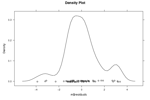
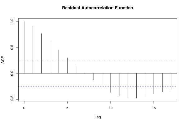
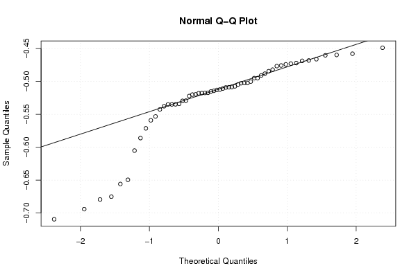
Title produced by software

Linear Regression Graphical Model Validation

Date of computation

Tue, 27 Oct 2009 13:42:59 -0600

Cite this page as follows

Statistical Computations at FreeStatistics.org, Office for Research Development and Education, URL https://freestatistics.org/blog/index.php?v=date/2009/Oct/27/t1256672648iznue1jd63wb14v.htm/, Retrieved Tue, 07 May 2024 22:34:24 +0000

Statistical Computations at FreeStatistics.org, Office for Research Development and Education, URL https://freestatistics.org/blog/index.php?pk=51181, Retrieved Tue, 07 May 2024 22:34:24 +0000

QR Codes:

Paste this QR Code to cite your computation.

Original text written by user:

IsPrivate?

No (this computation is public)

User-defined keywords

Estimated Impact

129

Family? (F = Feedback message, R = changed R code, M = changed R Module, P = changed Parameters, D = changed Data)

-       [Linear Regression Graphical Model Validation] [Workshop 4:Linear...] [2009-10-27 19:42:59] [a5c6be3c0aa55fdb2a703a08e16947ef] [Current]
-    D    [Linear Regression Graphical Model Validation] [Workshop 4:Linear...] [2009-10-27 20:24:52] [1433a524809eda02c3198b3ae6eebb69] 
-    D      [Linear Regression Graphical Model Validation] [Workshop 4 part 2...] [2009-10-28 16:52:46] [b6394cb5c2dcec6d17418d3cdf42d699] 
-    D      [Linear Regression Graphical Model Validation] [Workshop 4, Part ...] [2009-10-28 16:53:13] [aba88da643e3763d32ff92bd8f92a385] 
F    D      [Linear Regression Graphical Model Validation] [workshop 4 part 2] [2009-10-28 16:52:59] [af8eb90b4bf1bcfcc4325c143dbee260] 
-    D      [Linear Regression Graphical Model Validation] [Workshop 4 part 2...] [2009-10-28 17:03:12] [b6394cb5c2dcec6d17418d3cdf42d699] 

Feedback Forum

Post a new message

Dataseries X:

Download CSV

Histogram

Boxplots

-0,5349
-0,5348
-0,5591
-0,5200
-0,5173
-0,5153
-0,5048
-0,4950
-0,4597
-0,4681
-0,4909
-0,4579
-0,4758
-0,4662
-0,4821
-0,4767
-0,4740
-0,5295
-0,5075
-0,5222
-0,5377
-0,5108
-0,5197
-0,5292
-0,5024
-0,5175
-0,5088
-0,5180
-0,5177
-0,5027
-0,5002
-0,4882
-0,4603
-0,4687
-0,5092
-0,4729
-0,4488
-0,5085
-0,5142
-0,5130
-0,4721
-0,5425
-0,5123
-0,4845
-0,4950
-0,5024
-0,5349
-0,5861
-0,6495
-0,6751
-0,7095
-0,6941
-0,6794
-0,6559
-0,6051
-0,5713
-0,5532
-0,5341

Dataseries Y:

Download CSV

Histogram

2,55
2,27
2,26
2,57
3,07
2,76
2,51
2,87
3,14
3,11
3,16
2,47
2,57
2,89
2,63
2,38
1,69
1,96
2,19
1,87
1,60
1,63
1,22
1,21
1,49
1,64
1,66
1,77
1,82
1,78
1,28
1,29
1,37
1,12
1,51
2,24
2,94
3,09
3,46
3,64
4,39
4,15
5,21
5,80
5,91
5,39
5,46
4,72
3,14
2,63
2,32
1,93
0,62
0,60
-0,37
-1,10
-1,68
-0,78

Summary of computational transaction
Raw Input	view raw input (R code)
Raw Output	view raw output of R engine
Computing time	5 seconds
R Server	'RServer@AstonUniversity' @ vre.aston.ac.uk

\begin{tabular}{lllllllll}
\hline
Summary of computational transaction \tabularnewline
Raw Input & view raw input (R code)  \tabularnewline
Raw Output & view raw output of R engine  \tabularnewline
Computing time & 5 seconds \tabularnewline
R Server & 'RServer@AstonUniversity' @ vre.aston.ac.uk \tabularnewline
\hline
\end{tabular}
%Source: https://freestatistics.org/blog/index.php?pk=51181&T=0

[TABLE]
[ROW][C]Summary of computational transaction[/C][/ROW]
[ROW][C]Raw Input[/C][C]view raw input (R code) [/C][/ROW]
[ROW][C]Raw Output[/C][C]view raw output of R engine [/C][/ROW]
[ROW][C]Computing time[/C][C]5 seconds[/C][/ROW]
[ROW][C]R Server[/C][C]'RServer@AstonUniversity' @ vre.aston.ac.uk[/C][/ROW]
[/TABLE]
Source: https://freestatistics.org/blog/index.php?pk=51181&T=0

Globally Unique Identifier (entire table): ba.freestatistics.org/blog/index.php?pk=51181&T=0

As an alternative you can also use a QR Code:

The GUIDs for individual cells are displayed in the table below:

Summary of computational transaction
Raw Input	view raw input (R code)
Raw Output	view raw output of R engine
Computing time	5 seconds
R Server	'RServer@AstonUniversity' @ vre.aston.ac.uk

Simple Linear Regression
Statistics	Estimate	S.D.	T-STAT (H0: coeff=0)	P-value (two-sided)
constant term	5.34739038623997	1.75667071229312	3.04404823785079	0.00355214640651891
slope	5.67685147216042	3.31912086219865	1.71034792279302	0.0927370124118139

\begin{tabular}{lllllllll}
\hline
Simple Linear Regression \tabularnewline
Statistics & Estimate & S.D. & T-STAT (H0: coeff=0) & P-value (two-sided) \tabularnewline
constant term & 5.34739038623997 & 1.75667071229312 & 3.04404823785079 & 0.00355214640651891 \tabularnewline
slope & 5.67685147216042 & 3.31912086219865 & 1.71034792279302 & 0.0927370124118139 \tabularnewline
\hline
\end{tabular}
%Source: https://freestatistics.org/blog/index.php?pk=51181&T=1

[TABLE]
[ROW][C]Simple Linear Regression[/C][/ROW]
[ROW][C]Statistics[/C][C]Estimate[/C][C]S.D.[/C][C]T-STAT (H0: coeff=0)[/C][C]P-value (two-sided)[/C][/ROW]
[ROW][C]constant term[/C][C]5.34739038623997[/C][C]1.75667071229312[/C][C]3.04404823785079[/C][C]0.00355214640651891[/C][/ROW]
[ROW][C]slope[/C][C]5.67685147216042[/C][C]3.31912086219865[/C][C]1.71034792279302[/C][C]0.0927370124118139[/C][/ROW]
[/TABLE]
Source: https://freestatistics.org/blog/index.php?pk=51181&T=1

Globally Unique Identifier (entire table): ba.freestatistics.org/blog/index.php?pk=51181&T=1

As an alternative you can also use a QR Code:

The GUIDs for individual cells are displayed in the table below:

Simple Linear Regression
Statistics	Estimate	S.D.	T-STAT (H0: coeff=0)	P-value (two-sided)
constant term	5.34739038623997	1.75667071229312	3.04404823785079	0.00355214640651891
slope	5.67685147216042	3.31912086219865	1.71034792279302	0.0927370124118139

Figure 1

PNG link

Postscript link

PDF link

Figure 2

PNG link

Postscript link

PDF link

Figure 3

PNG link

Postscript link

PDF link

Figure 4

PNG link

Postscript link

PDF link

Figure 5

PNG link

Postscript link

PDF link

Figure 6

PNG link

Postscript link

PDF link

Figure 7

PNG link

Postscript link

PDF link

Figure 8

PNG link

Postscript link

PDF link

Figure 9

PNG link

Postscript link

PDF link

Parameters (Session):

par1 = 0 ;

Parameters (R input):

par1 = 0 ;

R code (references can be found in the software module):

par1 <- as.numeric(par1)
library(lattice)
z <- as.data.frame(cbind(x,y))
m <- lm(y~x)
summary(m)
bitmap(file='test1.png')
plot(z,main='Scatterplot, lowess, and regression line')
lines(lowess(z),col='red')
abline(m)
grid()
dev.off()
bitmap(file='test2.png')
m2 <- lm(m$fitted.values ~ x)
summary(m2)
z2 <- as.data.frame(cbind(x,m$fitted.values))
names(z2) <- list('x','Fitted')
plot(z2,main='Scatterplot, lowess, and regression line')
lines(lowess(z2),col='red')
abline(m2)
grid()
dev.off()
bitmap(file='test3.png')
m3 <- lm(m$residuals ~ x)
summary(m3)
z3 <- as.data.frame(cbind(x,m$residuals))
names(z3) <- list('x','Residuals')
plot(z3,main='Scatterplot, lowess, and regression line')
lines(lowess(z3),col='red')
abline(m3)
grid()
dev.off()
bitmap(file='test4.png')
m4 <- lm(m$fitted.values ~ m$residuals)
summary(m4)
z4 <- as.data.frame(cbind(m$residuals,m$fitted.values))
names(z4) <- list('Residuals','Fitted')
plot(z4,main='Scatterplot, lowess, and regression line')
lines(lowess(z4),col='red')
abline(m4)
grid()
dev.off()
bitmap(file='test5.png')
myr <- as.ts(m$residuals)
z5 <- as.data.frame(cbind(lag(myr,1),myr))
names(z5) <- list('Lagged Residuals','Residuals')
plot(z5,main='Lag plot')
m5 <- lm(z5)
summary(m5)
abline(m5)
grid()
dev.off()
bitmap(file='test6.png')
hist(m$residuals,main='Residual Histogram',xlab='Residuals')
dev.off()
bitmap(file='test7.png')
if (par1 > 0)
{
densityplot(~m$residuals,col='black',main=paste('Density Plot   bw = ',par1),bw=par1)
} else {
densityplot(~m$residuals,col='black',main='Density Plot')
}
dev.off()
bitmap(file='test8.png')
acf(m$residuals,main='Residual Autocorrelation Function')
dev.off()
bitmap(file='test9.png')
qqnorm(x)
qqline(x)
grid()
dev.off()
load(file='createtable')
a<-table.start()
a<-table.row.start(a)
a<-table.element(a,'Simple Linear Regression',5,TRUE)
a<-table.row.end(a)
a<-table.row.start(a)
a<-table.element(a,'Statistics',1,TRUE)
a<-table.element(a,'Estimate',1,TRUE)
a<-table.element(a,'S.D.',1,TRUE)
a<-table.element(a,'T-STAT (H0: coeff=0)',1,TRUE)
a<-table.element(a,'P-value (two-sided)',1,TRUE)
a<-table.row.end(a)
a<-table.row.start(a)
a<-table.element(a,'constant term',header=TRUE)
a<-table.element(a,m$coefficients[[1]])
sd <- sqrt(vcov(m)[1,1])
a<-table.element(a,sd)
tstat <- m$coefficients[[1]]/sd
a<-table.element(a,tstat)
pval <- 2*(1-pt(abs(tstat),length(x)-2))
a<-table.element(a,pval)
a<-table.row.end(a)
a<-table.row.start(a)
a<-table.element(a,'slope',header=TRUE)
a<-table.element(a,m$coefficients[[2]])
sd <- sqrt(vcov(m)[2,2])
a<-table.element(a,sd)
tstat <- m$coefficients[[2]]/sd
a<-table.element(a,tstat)
pval <- 2*(1-pt(abs(tstat),length(x)-2))
a<-table.element(a,pval)
a<-table.row.end(a)
a<-table.end(a)
table.save(a,file='mytable.tab')

Free Statistics

Description of Statistical Computation

Tree of Dependent Computations

Dataset

Tables (Output of Computation)

Figures (Output of Computation)

Input Parameters & R Code