Free Statistics

of Irreproducible Research!

Author's title

Author*Unverified author*
R Software ModulePatrick.Wessarwasp_demand_forecasting_croston.wasp
Title produced by softwareCroston Forecasting
Date of computationThu, 13 May 2010 13:04:00 +0000
Cite this page as followsStatistical Computations at FreeStatistics.org, Office for Research Development and Education, URL https://freestatistics.org/blog/index.php?v=date/2010/May/13/t1273755878x3zkimsjs9lvugi.htm/, Retrieved Mon, 06 May 2024 10:13:05 +0000
Statistical Computations at FreeStatistics.org, Office for Research Development and Education, URL https://freestatistics.org/blog/index.php?pk=75917, Retrieved Mon, 06 May 2024 10:13:05 +0000
QR Codes:

Original text written by user:
IsPrivate?No (this computation is public)
User-defined keywordsB382,steven,coomans,thesis,ARIMA,Per2maand
Estimated Impact124
Family? (F = Feedback message, R = changed R code, M = changed R Module, P = changed Parameters, D = changed Data)
-       [Croston Forecasting] [B382,steven,cooma...] [2010-05-13 13:04:00] [d41d8cd98f00b204e9800998ecf8427e] [Current]
Feedback Forum

Post a new message
Dataseries X:
285
215.375
313.725
256.7625
273.79
173.0125
174.875
258.2625
222.65
231.7375
150.778
144.1375
136.15
152.875
238.375
147.8
35.425
80.375
143.375
194.8875
190.43
122.525
153.125
79.6
182.8625


Summary of computational transaction
Raw Inputview raw input (R code)
Raw Outputview raw output of R engine
Computing time3 seconds
R Serverwessa.org @ wessa.org

\begin{tabular}{lllllllll}
\hline
Summary of computational transaction \tabularnewline
Raw Input & view raw input (R code)  \tabularnewline
Raw Output & view raw output of R engine  \tabularnewline
Computing time & 3 seconds \tabularnewline
R Server & wessa.org @ wessa.org \tabularnewline
\hline
\end{tabular}
%Source: https://freestatistics.org/blog/index.php?pk=75917&T=0

[TABLE]
[ROW][C]Summary of computational transaction[/C][/ROW]
[ROW][C]Raw Input[/C][C]view raw input (R code) [/C][/ROW]
[ROW][C]Raw Output[/C][C]view raw output of R engine [/C][/ROW]
[ROW][C]Computing time[/C][C]3 seconds[/C][/ROW]
[ROW][C]R Server[/C][C]wessa.org @ wessa.org[/C][/ROW]
[/TABLE]
Source: https://freestatistics.org/blog/index.php?pk=75917&T=0

Globally Unique Identifier (entire table): ba.freestatistics.org/blog/index.php?pk=75917&T=0

As an alternative you can also use a QR Code:  

The GUIDs for individual cells are displayed in the table below:

Summary of computational transaction
Raw Inputview raw input (R code)
Raw Outputview raw output of R engine
Computing time3 seconds
R Serverwessa.org @ wessa.org


Demand Forecast
PointForecast95% LB80% LB80% UB95% UB
26145.46345979031831.283713026552270.8053362876409220.121583292994259.643206554083
27145.46345979031824.606993730332866.4396641965898224.487255384045266.319925850302
28145.46345979031818.280299718007262.3028613368575228.624058243777272.646619862628
29145.46345979031812.253749095302658.3623116909041232.564607889731278.673170485332
30145.4634597903186.4882899184291654.5924805651859236.334439015449284.438629662206
31145.4634597903180.95266898772416750.9729325908535239.953986989782289.974250592911
32145.463459790318-4.3785886335530247.4870106021019243.439908978533295.305508214188
33145.463459790318-9.5265730935173844.1209244923029246.805995088332300.453492674152
34145.463459790318-14.508978807094940.8631045054157250.063815075219305.43589838773
35145.463459790318-19.340823916974437.7037308057565253.223188774879310.267743497609
36145.463459790318-24.034984880258234.6343839305758256.292535650059314.961904460893
37145.463459790318-28.60260112683831.6477801981685259.279139382466319.529520707473
38145.463459790318-33.053386419460528.7375681204696262.189351460165323.980306000096
39145.463459790318-37.395871932611625.8981694623155265.028750118320328.322791513247
40145.463459790318-41.637598506066523.1246535336036267.802266047031332.564518086701
41145.463459790318-45.785270488075620.4126365966411270.514282983994336.712190068711
42145.463459790318-49.844880150833517.7582005152412273.168719065394340.771799731469
43145.463459790318-53.821809279021615.1578263295465275.769093251089344.748728859657
44145.463459790318-57.720912850664712.6083395400571278.318580040578348.6478324313
45145.463459790318-61.546588523720110.1068646727928280.820054907842352.473508104355
46145.463459790318-65.30283476469647.6507872710319283.276132309603356.229754345331
47145.463459790318-68.99329980919145.23772188173598285.689197698899359.920219389826
48145.463459790318-72.62132316207512.86548492003911288.061434660596363.54824274271
49145.463459790318-76.18997098137810.532071532966938290.394848047668367.116890562013

\begin{tabular}{lllllllll}
\hline
Demand Forecast \tabularnewline
Point & Forecast & 95% LB & 80% LB & 80% UB & 95% UB \tabularnewline
26 & 145.463459790318 & 31.2837130265522 & 70.8053362876409 & 220.121583292994 & 259.643206554083 \tabularnewline
27 & 145.463459790318 & 24.6069937303328 & 66.4396641965898 & 224.487255384045 & 266.319925850302 \tabularnewline
28 & 145.463459790318 & 18.2802997180072 & 62.3028613368575 & 228.624058243777 & 272.646619862628 \tabularnewline
29 & 145.463459790318 & 12.2537490953026 & 58.3623116909041 & 232.564607889731 & 278.673170485332 \tabularnewline
30 & 145.463459790318 & 6.48828991842916 & 54.5924805651859 & 236.334439015449 & 284.438629662206 \tabularnewline
31 & 145.463459790318 & 0.952668987724167 & 50.9729325908535 & 239.953986989782 & 289.974250592911 \tabularnewline
32 & 145.463459790318 & -4.37858863355302 & 47.4870106021019 & 243.439908978533 & 295.305508214188 \tabularnewline
33 & 145.463459790318 & -9.52657309351738 & 44.1209244923029 & 246.805995088332 & 300.453492674152 \tabularnewline
34 & 145.463459790318 & -14.5089788070949 & 40.8631045054157 & 250.063815075219 & 305.43589838773 \tabularnewline
35 & 145.463459790318 & -19.3408239169744 & 37.7037308057565 & 253.223188774879 & 310.267743497609 \tabularnewline
36 & 145.463459790318 & -24.0349848802582 & 34.6343839305758 & 256.292535650059 & 314.961904460893 \tabularnewline
37 & 145.463459790318 & -28.602601126838 & 31.6477801981685 & 259.279139382466 & 319.529520707473 \tabularnewline
38 & 145.463459790318 & -33.0533864194605 & 28.7375681204696 & 262.189351460165 & 323.980306000096 \tabularnewline
39 & 145.463459790318 & -37.3958719326116 & 25.8981694623155 & 265.028750118320 & 328.322791513247 \tabularnewline
40 & 145.463459790318 & -41.6375985060665 & 23.1246535336036 & 267.802266047031 & 332.564518086701 \tabularnewline
41 & 145.463459790318 & -45.7852704880756 & 20.4126365966411 & 270.514282983994 & 336.712190068711 \tabularnewline
42 & 145.463459790318 & -49.8448801508335 & 17.7582005152412 & 273.168719065394 & 340.771799731469 \tabularnewline
43 & 145.463459790318 & -53.8218092790216 & 15.1578263295465 & 275.769093251089 & 344.748728859657 \tabularnewline
44 & 145.463459790318 & -57.7209128506647 & 12.6083395400571 & 278.318580040578 & 348.6478324313 \tabularnewline
45 & 145.463459790318 & -61.5465885237201 & 10.1068646727928 & 280.820054907842 & 352.473508104355 \tabularnewline
46 & 145.463459790318 & -65.3028347646964 & 7.6507872710319 & 283.276132309603 & 356.229754345331 \tabularnewline
47 & 145.463459790318 & -68.9932998091914 & 5.23772188173598 & 285.689197698899 & 359.920219389826 \tabularnewline
48 & 145.463459790318 & -72.6213231620751 & 2.86548492003911 & 288.061434660596 & 363.54824274271 \tabularnewline
49 & 145.463459790318 & -76.1899709813781 & 0.532071532966938 & 290.394848047668 & 367.116890562013 \tabularnewline
\hline
\end{tabular}
%Source: https://freestatistics.org/blog/index.php?pk=75917&T=1

[TABLE]
[ROW][C]Demand Forecast[/C][/ROW]
[ROW][C]Point[/C][C]Forecast[/C][C]95% LB[/C][C]80% LB[/C][C]80% UB[/C][C]95% UB[/C][/ROW]
[ROW][C]26[/C][C]145.463459790318[/C][C]31.2837130265522[/C][C]70.8053362876409[/C][C]220.121583292994[/C][C]259.643206554083[/C][/ROW]
[ROW][C]27[/C][C]145.463459790318[/C][C]24.6069937303328[/C][C]66.4396641965898[/C][C]224.487255384045[/C][C]266.319925850302[/C][/ROW]
[ROW][C]28[/C][C]145.463459790318[/C][C]18.2802997180072[/C][C]62.3028613368575[/C][C]228.624058243777[/C][C]272.646619862628[/C][/ROW]
[ROW][C]29[/C][C]145.463459790318[/C][C]12.2537490953026[/C][C]58.3623116909041[/C][C]232.564607889731[/C][C]278.673170485332[/C][/ROW]
[ROW][C]30[/C][C]145.463459790318[/C][C]6.48828991842916[/C][C]54.5924805651859[/C][C]236.334439015449[/C][C]284.438629662206[/C][/ROW]
[ROW][C]31[/C][C]145.463459790318[/C][C]0.952668987724167[/C][C]50.9729325908535[/C][C]239.953986989782[/C][C]289.974250592911[/C][/ROW]
[ROW][C]32[/C][C]145.463459790318[/C][C]-4.37858863355302[/C][C]47.4870106021019[/C][C]243.439908978533[/C][C]295.305508214188[/C][/ROW]
[ROW][C]33[/C][C]145.463459790318[/C][C]-9.52657309351738[/C][C]44.1209244923029[/C][C]246.805995088332[/C][C]300.453492674152[/C][/ROW]
[ROW][C]34[/C][C]145.463459790318[/C][C]-14.5089788070949[/C][C]40.8631045054157[/C][C]250.063815075219[/C][C]305.43589838773[/C][/ROW]
[ROW][C]35[/C][C]145.463459790318[/C][C]-19.3408239169744[/C][C]37.7037308057565[/C][C]253.223188774879[/C][C]310.267743497609[/C][/ROW]
[ROW][C]36[/C][C]145.463459790318[/C][C]-24.0349848802582[/C][C]34.6343839305758[/C][C]256.292535650059[/C][C]314.961904460893[/C][/ROW]
[ROW][C]37[/C][C]145.463459790318[/C][C]-28.602601126838[/C][C]31.6477801981685[/C][C]259.279139382466[/C][C]319.529520707473[/C][/ROW]
[ROW][C]38[/C][C]145.463459790318[/C][C]-33.0533864194605[/C][C]28.7375681204696[/C][C]262.189351460165[/C][C]323.980306000096[/C][/ROW]
[ROW][C]39[/C][C]145.463459790318[/C][C]-37.3958719326116[/C][C]25.8981694623155[/C][C]265.028750118320[/C][C]328.322791513247[/C][/ROW]
[ROW][C]40[/C][C]145.463459790318[/C][C]-41.6375985060665[/C][C]23.1246535336036[/C][C]267.802266047031[/C][C]332.564518086701[/C][/ROW]
[ROW][C]41[/C][C]145.463459790318[/C][C]-45.7852704880756[/C][C]20.4126365966411[/C][C]270.514282983994[/C][C]336.712190068711[/C][/ROW]
[ROW][C]42[/C][C]145.463459790318[/C][C]-49.8448801508335[/C][C]17.7582005152412[/C][C]273.168719065394[/C][C]340.771799731469[/C][/ROW]
[ROW][C]43[/C][C]145.463459790318[/C][C]-53.8218092790216[/C][C]15.1578263295465[/C][C]275.769093251089[/C][C]344.748728859657[/C][/ROW]
[ROW][C]44[/C][C]145.463459790318[/C][C]-57.7209128506647[/C][C]12.6083395400571[/C][C]278.318580040578[/C][C]348.6478324313[/C][/ROW]
[ROW][C]45[/C][C]145.463459790318[/C][C]-61.5465885237201[/C][C]10.1068646727928[/C][C]280.820054907842[/C][C]352.473508104355[/C][/ROW]
[ROW][C]46[/C][C]145.463459790318[/C][C]-65.3028347646964[/C][C]7.6507872710319[/C][C]283.276132309603[/C][C]356.229754345331[/C][/ROW]
[ROW][C]47[/C][C]145.463459790318[/C][C]-68.9932998091914[/C][C]5.23772188173598[/C][C]285.689197698899[/C][C]359.920219389826[/C][/ROW]
[ROW][C]48[/C][C]145.463459790318[/C][C]-72.6213231620751[/C][C]2.86548492003911[/C][C]288.061434660596[/C][C]363.54824274271[/C][/ROW]
[ROW][C]49[/C][C]145.463459790318[/C][C]-76.1899709813781[/C][C]0.532071532966938[/C][C]290.394848047668[/C][C]367.116890562013[/C][/ROW]
[/TABLE]
Source: https://freestatistics.org/blog/index.php?pk=75917&T=1

Globally Unique Identifier (entire table): ba.freestatistics.org/blog/index.php?pk=75917&T=1

As an alternative you can also use a QR Code:  

The GUIDs for individual cells are displayed in the table below:

Demand Forecast
PointForecast95% LB80% LB80% UB95% UB
26145.46345979031831.283713026552270.8053362876409220.121583292994259.643206554083
27145.46345979031824.606993730332866.4396641965898224.487255384045266.319925850302
28145.46345979031818.280299718007262.3028613368575228.624058243777272.646619862628
29145.46345979031812.253749095302658.3623116909041232.564607889731278.673170485332
30145.4634597903186.4882899184291654.5924805651859236.334439015449284.438629662206
31145.4634597903180.95266898772416750.9729325908535239.953986989782289.974250592911
32145.463459790318-4.3785886335530247.4870106021019243.439908978533295.305508214188
33145.463459790318-9.5265730935173844.1209244923029246.805995088332300.453492674152
34145.463459790318-14.508978807094940.8631045054157250.063815075219305.43589838773
35145.463459790318-19.340823916974437.7037308057565253.223188774879310.267743497609
36145.463459790318-24.034984880258234.6343839305758256.292535650059314.961904460893
37145.463459790318-28.60260112683831.6477801981685259.279139382466319.529520707473
38145.463459790318-33.053386419460528.7375681204696262.189351460165323.980306000096
39145.463459790318-37.395871932611625.8981694623155265.028750118320328.322791513247
40145.463459790318-41.637598506066523.1246535336036267.802266047031332.564518086701
41145.463459790318-45.785270488075620.4126365966411270.514282983994336.712190068711
42145.463459790318-49.844880150833517.7582005152412273.168719065394340.771799731469
43145.463459790318-53.821809279021615.1578263295465275.769093251089344.748728859657
44145.463459790318-57.720912850664712.6083395400571278.318580040578348.6478324313
45145.463459790318-61.546588523720110.1068646727928280.820054907842352.473508104355
46145.463459790318-65.30283476469647.6507872710319283.276132309603356.229754345331
47145.463459790318-68.99329980919145.23772188173598285.689197698899359.920219389826
48145.463459790318-72.62132316207512.86548492003911288.061434660596363.54824274271
49145.463459790318-76.18997098137810.532071532966938290.394848047668367.116890562013


Actuals and Interpolation
TimeActualForecast
1285284.715000203273
2215.375273.669961695715
3313.725251.121344746975
4256.7625274.792708736568
5273.79268.316598141974
6173.0125269.853519048767
7174.875235.891289968433
8258.2625214.685176171976
9222.65229.822804324978
10231.7375227.333358752735
11150.778228.857278044667
12144.1375201.763796135814
13136.15181.769285845826
14152.875165.941563187890
15238.375161.40829991438
16147.8188.11152745539
1735.425174.125600162880
1880.375126.004166756322
19143.375110.173380876921
20194.8875121.692499793419
21190.43147.087096517147
22122.525162.124674010416
23153.125148.385789010579
2479.6150.030031637519
25182.8625125.594727004357

\begin{tabular}{lllllllll}
\hline
Actuals and Interpolation \tabularnewline
Time & Actual & Forecast \tabularnewline
1 & 285 & 284.715000203273 \tabularnewline
2 & 215.375 & 273.669961695715 \tabularnewline
3 & 313.725 & 251.121344746975 \tabularnewline
4 & 256.7625 & 274.792708736568 \tabularnewline
5 & 273.79 & 268.316598141974 \tabularnewline
6 & 173.0125 & 269.853519048767 \tabularnewline
7 & 174.875 & 235.891289968433 \tabularnewline
8 & 258.2625 & 214.685176171976 \tabularnewline
9 & 222.65 & 229.822804324978 \tabularnewline
10 & 231.7375 & 227.333358752735 \tabularnewline
11 & 150.778 & 228.857278044667 \tabularnewline
12 & 144.1375 & 201.763796135814 \tabularnewline
13 & 136.15 & 181.769285845826 \tabularnewline
14 & 152.875 & 165.941563187890 \tabularnewline
15 & 238.375 & 161.40829991438 \tabularnewline
16 & 147.8 & 188.11152745539 \tabularnewline
17 & 35.425 & 174.125600162880 \tabularnewline
18 & 80.375 & 126.004166756322 \tabularnewline
19 & 143.375 & 110.173380876921 \tabularnewline
20 & 194.8875 & 121.692499793419 \tabularnewline
21 & 190.43 & 147.087096517147 \tabularnewline
22 & 122.525 & 162.124674010416 \tabularnewline
23 & 153.125 & 148.385789010579 \tabularnewline
24 & 79.6 & 150.030031637519 \tabularnewline
25 & 182.8625 & 125.594727004357 \tabularnewline
\hline
\end{tabular}
%Source: https://freestatistics.org/blog/index.php?pk=75917&T=2

[TABLE]
[ROW][C]Actuals and Interpolation[/C][/ROW]
[ROW][C]Time[/C][C]Actual[/C][C]Forecast[/C][/ROW]
[ROW][C]1[/C][C]285[/C][C]284.715000203273[/C][/ROW]
[ROW][C]2[/C][C]215.375[/C][C]273.669961695715[/C][/ROW]
[ROW][C]3[/C][C]313.725[/C][C]251.121344746975[/C][/ROW]
[ROW][C]4[/C][C]256.7625[/C][C]274.792708736568[/C][/ROW]
[ROW][C]5[/C][C]273.79[/C][C]268.316598141974[/C][/ROW]
[ROW][C]6[/C][C]173.0125[/C][C]269.853519048767[/C][/ROW]
[ROW][C]7[/C][C]174.875[/C][C]235.891289968433[/C][/ROW]
[ROW][C]8[/C][C]258.2625[/C][C]214.685176171976[/C][/ROW]
[ROW][C]9[/C][C]222.65[/C][C]229.822804324978[/C][/ROW]
[ROW][C]10[/C][C]231.7375[/C][C]227.333358752735[/C][/ROW]
[ROW][C]11[/C][C]150.778[/C][C]228.857278044667[/C][/ROW]
[ROW][C]12[/C][C]144.1375[/C][C]201.763796135814[/C][/ROW]
[ROW][C]13[/C][C]136.15[/C][C]181.769285845826[/C][/ROW]
[ROW][C]14[/C][C]152.875[/C][C]165.941563187890[/C][/ROW]
[ROW][C]15[/C][C]238.375[/C][C]161.40829991438[/C][/ROW]
[ROW][C]16[/C][C]147.8[/C][C]188.11152745539[/C][/ROW]
[ROW][C]17[/C][C]35.425[/C][C]174.125600162880[/C][/ROW]
[ROW][C]18[/C][C]80.375[/C][C]126.004166756322[/C][/ROW]
[ROW][C]19[/C][C]143.375[/C][C]110.173380876921[/C][/ROW]
[ROW][C]20[/C][C]194.8875[/C][C]121.692499793419[/C][/ROW]
[ROW][C]21[/C][C]190.43[/C][C]147.087096517147[/C][/ROW]
[ROW][C]22[/C][C]122.525[/C][C]162.124674010416[/C][/ROW]
[ROW][C]23[/C][C]153.125[/C][C]148.385789010579[/C][/ROW]
[ROW][C]24[/C][C]79.6[/C][C]150.030031637519[/C][/ROW]
[ROW][C]25[/C][C]182.8625[/C][C]125.594727004357[/C][/ROW]
[/TABLE]
Source: https://freestatistics.org/blog/index.php?pk=75917&T=2

Globally Unique Identifier (entire table): ba.freestatistics.org/blog/index.php?pk=75917&T=2

As an alternative you can also use a QR Code:  

The GUIDs for individual cells are displayed in the table below:

Actuals and Interpolation
TimeActualForecast
1285284.715000203273
2215.375273.669961695715
3313.725251.121344746975
4256.7625274.792708736568
5273.79268.316598141974
6173.0125269.853519048767
7174.875235.891289968433
8258.2625214.685176171976
9222.65229.822804324978
10231.7375227.333358752735
11150.778228.857278044667
12144.1375201.763796135814
13136.15181.769285845826
14152.875165.941563187890
15238.375161.40829991438
16147.8188.11152745539
1735.425174.125600162880
1880.375126.004166756322
19143.375110.173380876921
20194.8875121.692499793419
21190.43147.087096517147
22122.525162.124674010416
23153.125148.385789010579
2479.6150.030031637519
25182.8625125.594727004357


\begin{tabular}{lllllllll}
\hline
What is next? \tabularnewline
Simulate Time Series \tabularnewline
Generate Forecasts \tabularnewline
Forecast Analysis \tabularnewline
\hline
\end{tabular}
%Source: https://freestatistics.org/blog/index.php?pk=75917&T=3

[TABLE]
[ROW][C]What is next?[/C][/ROW]
[ROW][C]Simulate Time Series[/C][/ROW]
[ROW][C]Generate Forecasts[/C][/ROW]
[ROW][C]Forecast Analysis[/C][/ROW]
[/TABLE]
Source: https://freestatistics.org/blog/index.php?pk=75917&T=3

Globally Unique Identifier (entire table): ba.freestatistics.org/blog/index.php?pk=75917&T=3

As an alternative you can also use a QR Code:  

The GUIDs for individual cells are displayed in the table below:

What is next?
Simulate Time Series
Generate Forecasts
Forecast Analysis


Parameters (Session):
par1 = Input box ; par2 = ARIMA ; par3 = NA ; par4 = NA ; par5 = ZZZ ; par6 = 12 ; par7 = dum ; par8 = dumresult ; par9 = 3 ; par10 = 0.1 ;
Parameters (R input):
par1 = Input box ; par2 = ARIMA ; par3 = NA ; par4 = NA ; par5 = ZZZ ; par6 = 12 ; par7 = dum ; par8 = dumresult ; par9 = 3 ; par10 = 0.1 ;
R code (references can be found in the software module):
if(par3!='NA') par3 <- as.numeric(par3) else par3 <- NA
if(par4!='NA') par4 <- as.numeric(par4) else par4 <- NA
par6 <- as.numeric(par6) #Seasonal Period
par9 <- as.numeric(par9) #Forecast Horizon
par10 <- as.numeric(par10) #Alpha
library(forecast)
if (par1 == 'CSV') {
xarr <- read.csv(file=paste('tmp/',par7,'.csv',sep=''),header=T)
numseries <- length(xarr[1,])-1
n <- length(xarr[,1])
nmh <- n - par9
nmhp1 <- nmh + 1
rarr <- array(NA,dim=c(n,numseries))
farr <- array(NA,dim=c(n,numseries))
parr <- array(NA,dim=c(numseries,8))
colnames(parr) = list('ME','RMSE','MAE','MPE','MAPE','MASE','ACF1','TheilU')
for(i in 1:numseries) {
sindex <- i+1
x <- xarr[,sindex]
if(par2=='Croston') {
if (i==1) m <- croston(x,alpha=par10)
if (i==1) mydemand <- m$model$demand[]
fit <- croston(x[1:nmh],h=par9,alpha=par10)
}
if(par2=='ARIMA') {
m <- auto.arima(ts(x,freq=par6),d=par3,D=par4)
mydemand <- forecast(m)
fit <- auto.arima(ts(x[1:nmh],freq=par6),d=par3,D=par4)
}
if(par2=='ETS') {
m <- ets(ts(x,freq=par6),model=par5)
mydemand <- forecast(m)
fit <- ets(ts(x[1:nmh],freq=par6),model=par5)
}
try(rarr[,i] <- mydemand$resid,silent=T)
try(farr[,i] <- mydemand$mean,silent=T)
if (par2!='Croston') parr[i,] <- accuracy(forecast(fit,par9),x[nmhp1:n])
if (par2=='Croston') parr[i,] <- accuracy(fit,x[nmhp1:n])
}
write.csv(farr,file=paste('tmp/',par8,'_f.csv',sep=''))
write.csv(rarr,file=paste('tmp/',par8,'_r.csv',sep=''))
write.csv(parr,file=paste('tmp/',par8,'_p.csv',sep=''))
}
if (par1 == 'Input box') {
numseries <- 1
n <- length(x)
if(par2=='Croston') {
m <- croston(x)
mydemand <- m$model$demand[]
}
if(par2=='ARIMA') {
m <- auto.arima(ts(x,freq=par6),d=par3,D=par4)
mydemand <- forecast(m)
}
if(par2=='ETS') {
m <- ets(ts(x,freq=par6),model=par5)
mydemand <- forecast(m)
}
summary(m)
}
bitmap(file='test1.png')
op <- par(mfrow=c(2,1))
if (par2=='Croston') plot(m)
if ((par2=='ARIMA') | par2=='ETS') plot(forecast(m))
plot(mydemand$resid,type='l',main='Residuals', ylab='residual value', xlab='time')
par(op)
dev.off()
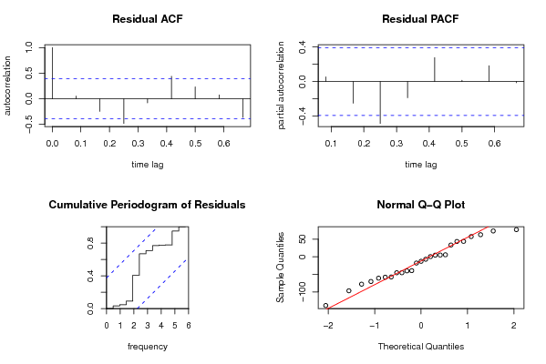
bitmap(file='pic2.png')
op <- par(mfrow=c(2,2))
acf(mydemand$resid, lag.max=n/3, main='Residual ACF', ylab='autocorrelation', xlab='time lag')
pacf(mydemand$resid,lag.max=n/3, main='Residual PACF', ylab='partial autocorrelation', xlab='time lag')
cpgram(mydemand$resid, main='Cumulative Periodogram of Residuals')
qqnorm(mydemand$resid); qqline(mydemand$resid, col=2)
par(op)
dev.off()
load(file='createtable')
a<-table.start()
a<-table.row.start(a)
a<-table.element(a,'Demand Forecast',6,TRUE)
a<-table.row.end(a)
a<-table.row.start(a)
a<-table.element(a,'Point',header=TRUE)
a<-table.element(a,'Forecast',header=TRUE)
a<-table.element(a,'95% LB',header=TRUE)
a<-table.element(a,'80% LB',header=TRUE)
a<-table.element(a,'80% UB',header=TRUE)
a<-table.element(a,'95% UB',header=TRUE)
a<-table.row.end(a)
for (i in 1:length(mydemand$mean)) {
a<-table.row.start(a)
a<-table.element(a,i+n,header=TRUE)
a<-table.element(a,as.numeric(mydemand$mean[i]))
a<-table.element(a,as.numeric(mydemand$lower[i,2]))
a<-table.element(a,as.numeric(mydemand$lower[i,1]))
a<-table.element(a,as.numeric(mydemand$upper[i,1]))
a<-table.element(a,as.numeric(mydemand$upper[i,2]))
a<-table.row.end(a)
}
a<-table.end(a)
table.save(a,file='mytable.tab')
a<-table.start()
a<-table.row.start(a)
a<-table.element(a,'Actuals and Interpolation',3,TRUE)
a<-table.row.end(a)
a<-table.row.start(a)
a<-table.element(a,'Time',header=TRUE)
a<-table.element(a,'Actual',header=TRUE)
a<-table.element(a,'Forecast',header=TRUE)
a<-table.row.end(a)
for (i in 1:n) {
a<-table.row.start(a)
a<-table.element(a,i,header=TRUE)
a<-table.element(a,x[i])
a<-table.element(a,x[i] - as.numeric(m$resid[i]))
a<-table.row.end(a)
}
a<-table.end(a)
table.save(a,file='mytable1.tab')
a<-table.start()
a<-table.row.start(a)
a<-table.element(a,'What is next?',1,TRUE)
a<-table.row.end(a)
a<-table.row.start(a)
a<-table.element(a,hyperlink(paste('https://automated.biganalytics.eu/Patrick.Wessa/rwasp_demand_forecasting_simulate.wasp',sep=''),'Simulate Time Series','',target=''))
a<-table.row.end(a)
a<-table.row.start(a)
a<-table.element(a,hyperlink(paste('https://automated.biganalytics.eu/Patrick.Wessa/rwasp_demand_forecasting_croston.wasp',sep=''),'Generate Forecasts','',target=''))
a<-table.row.end(a)
a<-table.row.start(a)
a<-table.element(a,hyperlink(paste('https://automated.biganalytics.eu/Patrick.Wessa/rwasp_demand_forecasting_analysis.wasp',sep=''),'Forecast Analysis','',target=''))
a<-table.row.end(a)
a<-table.end(a)
table.save(a,file='mytable0.tab')
-SERVER-wessa.org