Repository of Reproducible Computations

Free Statistics

of Irreproducible Research!

Author's title

Author

*The author of this computation has been verified*

R Software Module

rwasp_linear_regression.wasp

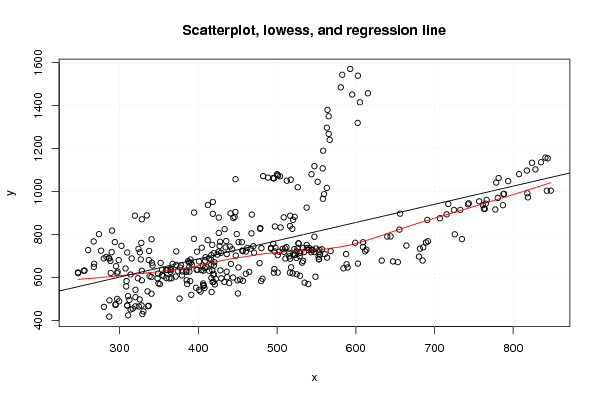
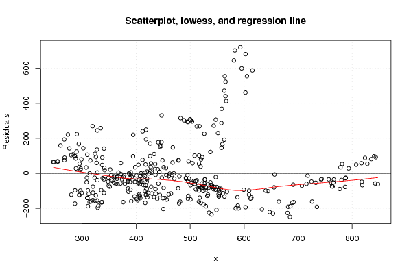
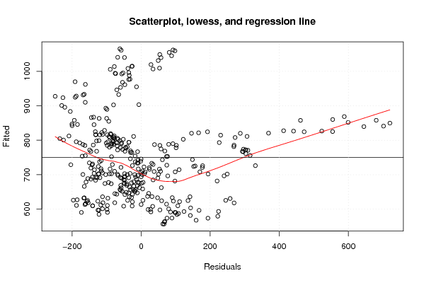
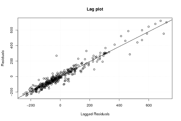
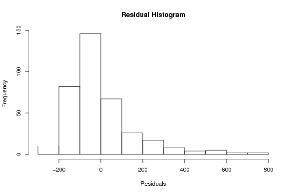
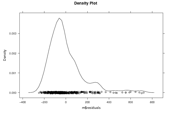
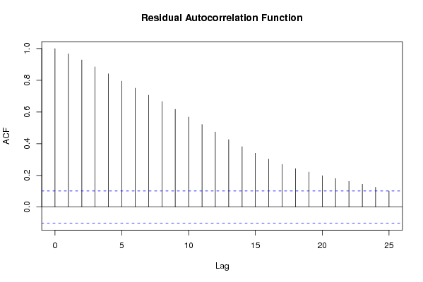
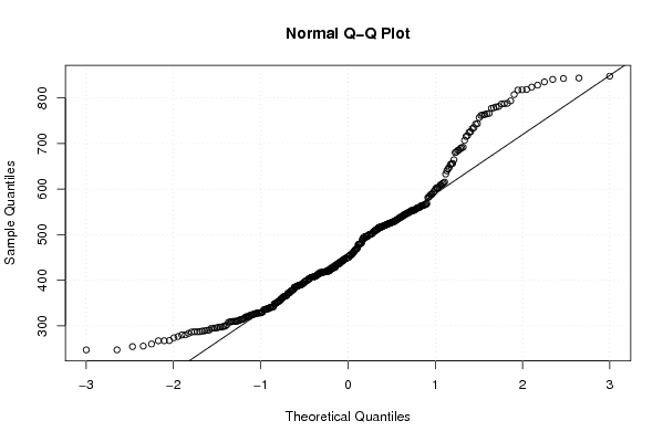
Title produced by software

Linear Regression Graphical Model Validation

Date of computation

Tue, 09 Nov 2010 15:50:28 +0000

Cite this page as follows

Statistical Computations at FreeStatistics.org, Office for Research Development and Education, URL https://freestatistics.org/blog/index.php?v=date/2010/Nov/09/t12893177567kxkjkozfho1rw1.htm/, Retrieved Sat, 27 Apr 2024 19:47:38 +0000

Statistical Computations at FreeStatistics.org, Office for Research Development and Education, URL https://freestatistics.org/blog/index.php?pk=92995, Retrieved Sat, 27 Apr 2024 19:47:38 +0000

QR Codes:

Paste this QR Code to cite your computation.

Original text written by user:

IsPrivate?

No (this computation is public)

User-defined keywords

Estimated Impact

119

Family? (F = Feedback message, R = changed R code, M = changed R Module, P = changed Parameters, D = changed Data)

-     [Linear Regression Graphical Model Validation] [Colombia Coffee -...] [2008-02-26 10:22:06] [74be16979710d4c4e7c6647856088456]
-  MPD    [Linear Regression Graphical Model Validation] [] [2010-11-09 15:50:28] [df17410ebb98883e83037e1662207ccb] [Current]

Feedback Forum

Post a new message

Dataseries X:

Download CSV

Histogram

Boxplots

Dataseries Y:

Download CSV

Histogram

Summary of computational transaction
Raw Input	view raw input (R code)
Raw Output	view raw output of R engine
Computing time	3 seconds
R Server	'George Udny Yule' @ 72.249.76.132

\begin{tabular}{lllllllll}
\hline
Summary of computational transaction \tabularnewline
Raw Input & view raw input (R code)  \tabularnewline
Raw Output & view raw output of R engine  \tabularnewline
Computing time & 3 seconds \tabularnewline
R Server & 'George Udny Yule' @ 72.249.76.132 \tabularnewline
\hline
\end{tabular}
%Source: https://freestatistics.org/blog/index.php?pk=92995&T=0

[TABLE]
[ROW][C]Summary of computational transaction[/C][/ROW]
[ROW][C]Raw Input[/C][C]view raw input (R code) [/C][/ROW]
[ROW][C]Raw Output[/C][C]view raw output of R engine [/C][/ROW]
[ROW][C]Computing time[/C][C]3 seconds[/C][/ROW]
[ROW][C]R Server[/C][C]'George Udny Yule' @ 72.249.76.132[/C][/ROW]
[/TABLE]
Source: https://freestatistics.org/blog/index.php?pk=92995&T=0

Globally Unique Identifier (entire table): ba.freestatistics.org/blog/index.php?pk=92995&T=0

As an alternative you can also use a QR Code:

The GUIDs for individual cells are displayed in the table below:

Summary of computational transaction
Raw Input	view raw input (R code)
Raw Output	view raw output of R engine
Computing time	3 seconds
R Server	'George Udny Yule' @ 72.249.76.132

Simple Linear Regression
Statistics	Estimate	S.D.	T-STAT (H0: coeff=0)	P-value (two-sided)
constant term	347.738690582509	30.2410462864513	11.4988974683163	0
slope	0.846477708632207	0.0610697019156163	13.8608455924975	0

\begin{tabular}{lllllllll}
\hline
Simple Linear Regression \tabularnewline
Statistics & Estimate & S.D. & T-STAT (H0: coeff=0) & P-value (two-sided) \tabularnewline
constant term & 347.738690582509 & 30.2410462864513 & 11.4988974683163 & 0 \tabularnewline
slope & 0.846477708632207 & 0.0610697019156163 & 13.8608455924975 & 0 \tabularnewline
\hline
\end{tabular}
%Source: https://freestatistics.org/blog/index.php?pk=92995&T=1

[TABLE]
[ROW][C]Simple Linear Regression[/C][/ROW]
[ROW][C]Statistics[/C][C]Estimate[/C][C]S.D.[/C][C]T-STAT (H0: coeff=0)[/C][C]P-value (two-sided)[/C][/ROW]
[ROW][C]constant term[/C][C]347.738690582509[/C][C]30.2410462864513[/C][C]11.4988974683163[/C][C]0[/C][/ROW]
[ROW][C]slope[/C][C]0.846477708632207[/C][C]0.0610697019156163[/C][C]13.8608455924975[/C][C]0[/C][/ROW]
[/TABLE]
Source: https://freestatistics.org/blog/index.php?pk=92995&T=1

Globally Unique Identifier (entire table): ba.freestatistics.org/blog/index.php?pk=92995&T=1

As an alternative you can also use a QR Code:

The GUIDs for individual cells are displayed in the table below:

Simple Linear Regression
Statistics	Estimate	S.D.	T-STAT (H0: coeff=0)	P-value (two-sided)
constant term	347.738690582509	30.2410462864513	11.4988974683163	0
slope	0.846477708632207	0.0610697019156163	13.8608455924975	0

Figure 1

PNG link

Postscript link

PDF link

Figure 2

PNG link

Postscript link

PDF link

Figure 3

PNG link

Postscript link

PDF link

Figure 4

PNG link

Postscript link

PDF link

Figure 5

PNG link

Postscript link

PDF link

Figure 6

PNG link

Postscript link

PDF link

Figure 7

PNG link

Postscript link

PDF link

Figure 8

PNG link

Postscript link

PDF link

Figure 9

PNG link

Postscript link

PDF link

Parameters (Session):

par1 = 12 ;

Parameters (R input):

par1 = 0 ;

R code (references can be found in the software module):

par1 <- as.numeric(par1)
library(lattice)
z <- as.data.frame(cbind(x,y))
m <- lm(y~x)
summary(m)
bitmap(file='test1.png')
plot(z,main='Scatterplot, lowess, and regression line')
lines(lowess(z),col='red')
abline(m)
grid()
dev.off()
bitmap(file='test2.png')
m2 <- lm(m$fitted.values ~ x)
summary(m2)
z2 <- as.data.frame(cbind(x,m$fitted.values))
names(z2) <- list('x','Fitted')
plot(z2,main='Scatterplot, lowess, and regression line')
lines(lowess(z2),col='red')
abline(m2)
grid()
dev.off()
bitmap(file='test3.png')
m3 <- lm(m$residuals ~ x)
summary(m3)
z3 <- as.data.frame(cbind(x,m$residuals))
names(z3) <- list('x','Residuals')
plot(z3,main='Scatterplot, lowess, and regression line')
lines(lowess(z3),col='red')
abline(m3)
grid()
dev.off()
bitmap(file='test4.png')
m4 <- lm(m$fitted.values ~ m$residuals)
summary(m4)
z4 <- as.data.frame(cbind(m$residuals,m$fitted.values))
names(z4) <- list('Residuals','Fitted')
plot(z4,main='Scatterplot, lowess, and regression line')
lines(lowess(z4),col='red')
abline(m4)
grid()
dev.off()
bitmap(file='test5.png')
myr <- as.ts(m$residuals)
z5 <- as.data.frame(cbind(lag(myr,1),myr))
names(z5) <- list('Lagged Residuals','Residuals')
plot(z5,main='Lag plot')
m5 <- lm(z5)
summary(m5)
abline(m5)
grid()
dev.off()
bitmap(file='test6.png')
hist(m$residuals,main='Residual Histogram',xlab='Residuals')
dev.off()
bitmap(file='test7.png')
if (par1 > 0)
{
densityplot(~m$residuals,col='black',main=paste('Density Plot   bw = ',par1),bw=par1)
} else {
densityplot(~m$residuals,col='black',main='Density Plot')
}
dev.off()
bitmap(file='test8.png')
acf(m$residuals,main='Residual Autocorrelation Function')
dev.off()
bitmap(file='test9.png')
qqnorm(x)
qqline(x)
grid()
dev.off()
load(file='createtable')
a<-table.start()
a<-table.row.start(a)
a<-table.element(a,'Simple Linear Regression',5,TRUE)
a<-table.row.end(a)
a<-table.row.start(a)
a<-table.element(a,'Statistics',1,TRUE)
a<-table.element(a,'Estimate',1,TRUE)
a<-table.element(a,'S.D.',1,TRUE)
a<-table.element(a,'T-STAT (H0: coeff=0)',1,TRUE)
a<-table.element(a,'P-value (two-sided)',1,TRUE)
a<-table.row.end(a)
a<-table.row.start(a)
a<-table.element(a,'constant term',header=TRUE)
a<-table.element(a,m$coefficients[[1]])
sd <- sqrt(vcov(m)[1,1])
a<-table.element(a,sd)
tstat <- m$coefficients[[1]]/sd
a<-table.element(a,tstat)
pval <- 2*(1-pt(abs(tstat),length(x)-2))
a<-table.element(a,pval)
a<-table.row.end(a)
a<-table.row.start(a)
a<-table.element(a,'slope',header=TRUE)
a<-table.element(a,m$coefficients[[2]])
sd <- sqrt(vcov(m)[2,2])
a<-table.element(a,sd)
tstat <- m$coefficients[[2]]/sd
a<-table.element(a,tstat)
pval <- 2*(1-pt(abs(tstat),length(x)-2))
a<-table.element(a,pval)
a<-table.row.end(a)
a<-table.end(a)
table.save(a,file='mytable.tab')

Free Statistics

Description of Statistical Computation

Tree of Dependent Computations

Dataset

Tables (Output of Computation)

Figures (Output of Computation)

Input Parameters & R Code