Repository of Reproducible Computations

Free Statistics

of Irreproducible Research!

Author's title

Author

*The author of this computation has been verified*

R Software Module

rwasp_autocorrelation.wasp

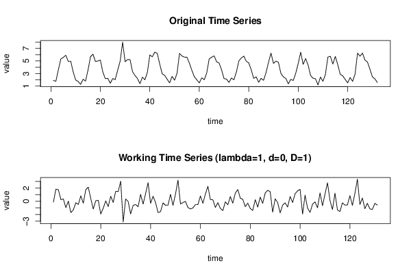
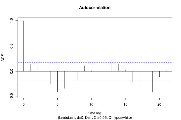
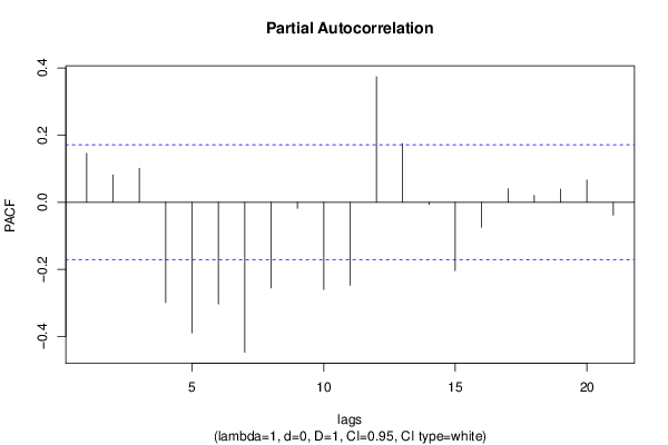
Title produced by software

(Partial) Autocorrelation Function

Date of computation

Sun, 16 Dec 2012 14:35:42 -0500

Cite this page as follows

Statistical Computations at FreeStatistics.org, Office for Research Development and Education, URL https://freestatistics.org/blog/index.php?v=date/2012/Dec/16/t1355687071hro0cxo8mrfrjwd.htm/, Retrieved Sun, 28 Apr 2024 18:12:38 +0000

Statistical Computations at FreeStatistics.org, Office for Research Development and Education, URL https://freestatistics.org/blog/index.php?pk=200561, Retrieved Sun, 28 Apr 2024 18:12:38 +0000

QR Codes:

Paste this QR Code to cite your computation.

Original text written by user:

IsPrivate?

No (this computation is public)

User-defined keywords

Estimated Impact

Family? (F = Feedback message, R = changed R code, M = changed R Module, P = changed Parameters, D = changed Data)

-     [Univariate Explorative Data Analysis] [Run Sequence gebo...] [2008-12-12 13:32:37] [76963dc1903f0f612b6153510a3818cf]
- R  D  [Univariate Explorative Data Analysis] [Run Sequence gebo...] [2008-12-17 12:14:40] [76963dc1903f0f612b6153510a3818cf]
-         [Univariate Explorative Data Analysis] [Run Sequence Plot...] [2008-12-22 18:19:51] [1ce0d16c8f4225c977b42c8fa93bc163]
- RMP       [Univariate Data Series] [Identifying Integ...] [2009-11-22 12:08:06] [b98453cac15ba1066b407e146608df68]
- R PD        [Univariate Data Series] [Paper : tijdreeks...] [2012-12-16 12:14:11] [5423d5951ef739cb88e60f5b30c308a9]
- RMPD            [(Partial) Autocorrelation Function] [paper ACF d=0 D=1] [2012-12-16 19:35:42] [292b44c97cfd231f70174a072f53fc18] [Current]

Feedback Forum

Post a new message

Dataseries X:

Download CSV

Histogram

Boxplots

Summary of computational transaction
Raw Input	view raw input (R code)
Raw Output	view raw output of R engine
Computing time	2 seconds
R Server	'Herman Ole Andreas Wold' @ wold.wessa.net

\begin{tabular}{lllllllll}
\hline
Summary of computational transaction \tabularnewline
Raw Input & view raw input (R code)  \tabularnewline
Raw Output & view raw output of R engine  \tabularnewline
Computing time & 2 seconds \tabularnewline
R Server & 'Herman Ole Andreas Wold' @ wold.wessa.net \tabularnewline
\hline
\end{tabular}
%Source: https://freestatistics.org/blog/index.php?pk=200561&T=0

[TABLE]
[ROW][C]Summary of computational transaction[/C][/ROW]
[ROW][C]Raw Input[/C][C]view raw input (R code) [/C][/ROW]
[ROW][C]Raw Output[/C][C]view raw output of R engine [/C][/ROW]
[ROW][C]Computing time[/C][C]2 seconds[/C][/ROW]
[ROW][C]R Server[/C][C]'Herman Ole Andreas Wold' @ wold.wessa.net[/C][/ROW]
[/TABLE]
Source: https://freestatistics.org/blog/index.php?pk=200561&T=0

Globally Unique Identifier (entire table): ba.freestatistics.org/blog/index.php?pk=200561&T=0

As an alternative you can also use a QR Code:

The GUIDs for individual cells are displayed in the table below:

Summary of computational transaction
Raw Input	view raw input (R code)
Raw Output	view raw output of R engine
Computing time	2 seconds
R Server	'Herman Ole Andreas Wold' @ wold.wessa.net

Autocorrelation Function
Time lag k	ACF(k)	T-STAT	P-value
1	0.145816	1.6689	0.048759
2	0.100794	1.1536	0.125374
3	0.123685	1.4156	0.079627
4	-0.250717	-2.8696	0.002397
5	-0.398781	-4.5643	6e-06
6	-0.336088	-3.8467	9.3e-05
7	-0.466249	-5.3365	0
8	-0.178508	-2.0431	0.021523
9	0.11142	1.2753	0.102237
10	0.012281	0.1406	0.444215
11	0.294433	3.3699	0.000494
12	0.691208	7.9112	0
13	0.222636	2.5482	0.005991
14	0.150509	1.7227	0.043655
15	0.033673	0.3854	0.350279
16	-0.217887	-2.4938	0.006941
17	-0.29841	-3.4155	0.000424
18	-0.361059	-4.1325	3.2e-05
19	-0.411485	-4.7097	3e-06
20	-0.106507	-1.219	0.112512
21	0.033917	0.3882	0.349249

\begin{tabular}{lllllllll}
\hline
Autocorrelation Function \tabularnewline
Time lag k & ACF(k) & T-STAT & P-value \tabularnewline
1 & 0.145816 & 1.6689 & 0.048759 \tabularnewline
2 & 0.100794 & 1.1536 & 0.125374 \tabularnewline
3 & 0.123685 & 1.4156 & 0.079627 \tabularnewline
4 & -0.250717 & -2.8696 & 0.002397 \tabularnewline
5 & -0.398781 & -4.5643 & 6e-06 \tabularnewline
6 & -0.336088 & -3.8467 & 9.3e-05 \tabularnewline
7 & -0.466249 & -5.3365 & 0 \tabularnewline
8 & -0.178508 & -2.0431 & 0.021523 \tabularnewline
9 & 0.11142 & 1.2753 & 0.102237 \tabularnewline
10 & 0.012281 & 0.1406 & 0.444215 \tabularnewline
11 & 0.294433 & 3.3699 & 0.000494 \tabularnewline
12 & 0.691208 & 7.9112 & 0 \tabularnewline
13 & 0.222636 & 2.5482 & 0.005991 \tabularnewline
14 & 0.150509 & 1.7227 & 0.043655 \tabularnewline
15 & 0.033673 & 0.3854 & 0.350279 \tabularnewline
16 & -0.217887 & -2.4938 & 0.006941 \tabularnewline
17 & -0.29841 & -3.4155 & 0.000424 \tabularnewline
18 & -0.361059 & -4.1325 & 3.2e-05 \tabularnewline
19 & -0.411485 & -4.7097 & 3e-06 \tabularnewline
20 & -0.106507 & -1.219 & 0.112512 \tabularnewline
21 & 0.033917 & 0.3882 & 0.349249 \tabularnewline
\hline
\end{tabular}
%Source: https://freestatistics.org/blog/index.php?pk=200561&T=1

[TABLE]
[ROW][C]Autocorrelation Function[/C][/ROW]
[ROW][C]Time lag k[/C][C]ACF(k)[/C][C]T-STAT[/C][C]P-value[/C][/ROW]
[ROW][C]1[/C][C]0.145816[/C][C]1.6689[/C][C]0.048759[/C][/ROW]
[ROW][C]2[/C][C]0.100794[/C][C]1.1536[/C][C]0.125374[/C][/ROW]
[ROW][C]3[/C][C]0.123685[/C][C]1.4156[/C][C]0.079627[/C][/ROW]
[ROW][C]4[/C][C]-0.250717[/C][C]-2.8696[/C][C]0.002397[/C][/ROW]
[ROW][C]5[/C][C]-0.398781[/C][C]-4.5643[/C][C]6e-06[/C][/ROW]
[ROW][C]6[/C][C]-0.336088[/C][C]-3.8467[/C][C]9.3e-05[/C][/ROW]
[ROW][C]7[/C][C]-0.466249[/C][C]-5.3365[/C][C]0[/C][/ROW]
[ROW][C]8[/C][C]-0.178508[/C][C]-2.0431[/C][C]0.021523[/C][/ROW]
[ROW][C]9[/C][C]0.11142[/C][C]1.2753[/C][C]0.102237[/C][/ROW]
[ROW][C]10[/C][C]0.012281[/C][C]0.1406[/C][C]0.444215[/C][/ROW]
[ROW][C]11[/C][C]0.294433[/C][C]3.3699[/C][C]0.000494[/C][/ROW]
[ROW][C]12[/C][C]0.691208[/C][C]7.9112[/C][C]0[/C][/ROW]
[ROW][C]13[/C][C]0.222636[/C][C]2.5482[/C][C]0.005991[/C][/ROW]
[ROW][C]14[/C][C]0.150509[/C][C]1.7227[/C][C]0.043655[/C][/ROW]
[ROW][C]15[/C][C]0.033673[/C][C]0.3854[/C][C]0.350279[/C][/ROW]
[ROW][C]16[/C][C]-0.217887[/C][C]-2.4938[/C][C]0.006941[/C][/ROW]
[ROW][C]17[/C][C]-0.29841[/C][C]-3.4155[/C][C]0.000424[/C][/ROW]
[ROW][C]18[/C][C]-0.361059[/C][C]-4.1325[/C][C]3.2e-05[/C][/ROW]
[ROW][C]19[/C][C]-0.411485[/C][C]-4.7097[/C][C]3e-06[/C][/ROW]
[ROW][C]20[/C][C]-0.106507[/C][C]-1.219[/C][C]0.112512[/C][/ROW]
[ROW][C]21[/C][C]0.033917[/C][C]0.3882[/C][C]0.349249[/C][/ROW]
[/TABLE]
Source: https://freestatistics.org/blog/index.php?pk=200561&T=1

Globally Unique Identifier (entire table): ba.freestatistics.org/blog/index.php?pk=200561&T=1

As an alternative you can also use a QR Code:

The GUIDs for individual cells are displayed in the table below:

Autocorrelation Function
Time lag k	ACF(k)	T-STAT	P-value
1	0.145816	1.6689	0.048759
2	0.100794	1.1536	0.125374
3	0.123685	1.4156	0.079627
4	-0.250717	-2.8696	0.002397
5	-0.398781	-4.5643	6e-06
6	-0.336088	-3.8467	9.3e-05
7	-0.466249	-5.3365	0
8	-0.178508	-2.0431	0.021523
9	0.11142	1.2753	0.102237
10	0.012281	0.1406	0.444215
11	0.294433	3.3699	0.000494
12	0.691208	7.9112	0
13	0.222636	2.5482	0.005991
14	0.150509	1.7227	0.043655
15	0.033673	0.3854	0.350279
16	-0.217887	-2.4938	0.006941
17	-0.29841	-3.4155	0.000424
18	-0.361059	-4.1325	3.2e-05
19	-0.411485	-4.7097	3e-06
20	-0.106507	-1.219	0.112512
21	0.033917	0.3882	0.349249

Partial Autocorrelation Function
Time lag k	PACF(k)	T-STAT	P-value
1	0.145816	1.6689	0.048759
2	0.081259	0.9301	0.177027
3	0.101137	1.1576	0.124573
4	-0.29911	-3.4235	0.000413
5	-0.389074	-4.4532	9e-06
6	-0.303027	-3.4683	0.000355
7	-0.447042	-5.1166	1e-06
8	-0.255452	-2.9238	0.002038
9	-0.01842	-0.2108	0.416677
10	-0.259991	-2.9757	0.001741
11	-0.247617	-2.8341	0.002662
12	0.374004	4.2807	1.8e-05
13	0.175127	2.0044	0.023543
14	-0.006542	-0.0749	0.470215
15	-0.20401	-2.335	0.010532
16	-0.074496	-0.8527	0.197704
17	0.04037	0.4621	0.322403
18	0.020497	0.2346	0.407443
19	0.039043	0.4469	0.327854
20	0.066054	0.756	0.225495
21	-0.038485	-0.4405	0.330158

\begin{tabular}{lllllllll}
\hline
Partial Autocorrelation Function \tabularnewline
Time lag k & PACF(k) & T-STAT & P-value \tabularnewline
1 & 0.145816 & 1.6689 & 0.048759 \tabularnewline
2 & 0.081259 & 0.9301 & 0.177027 \tabularnewline
3 & 0.101137 & 1.1576 & 0.124573 \tabularnewline
4 & -0.29911 & -3.4235 & 0.000413 \tabularnewline
5 & -0.389074 & -4.4532 & 9e-06 \tabularnewline
6 & -0.303027 & -3.4683 & 0.000355 \tabularnewline
7 & -0.447042 & -5.1166 & 1e-06 \tabularnewline
8 & -0.255452 & -2.9238 & 0.002038 \tabularnewline
9 & -0.01842 & -0.2108 & 0.416677 \tabularnewline
10 & -0.259991 & -2.9757 & 0.001741 \tabularnewline
11 & -0.247617 & -2.8341 & 0.002662 \tabularnewline
12 & 0.374004 & 4.2807 & 1.8e-05 \tabularnewline
13 & 0.175127 & 2.0044 & 0.023543 \tabularnewline
14 & -0.006542 & -0.0749 & 0.470215 \tabularnewline
15 & -0.20401 & -2.335 & 0.010532 \tabularnewline
16 & -0.074496 & -0.8527 & 0.197704 \tabularnewline
17 & 0.04037 & 0.4621 & 0.322403 \tabularnewline
18 & 0.020497 & 0.2346 & 0.407443 \tabularnewline
19 & 0.039043 & 0.4469 & 0.327854 \tabularnewline
20 & 0.066054 & 0.756 & 0.225495 \tabularnewline
21 & -0.038485 & -0.4405 & 0.330158 \tabularnewline
\hline
\end{tabular}
%Source: https://freestatistics.org/blog/index.php?pk=200561&T=2

[TABLE]
[ROW][C]Partial Autocorrelation Function[/C][/ROW]
[ROW][C]Time lag k[/C][C]PACF(k)[/C][C]T-STAT[/C][C]P-value[/C][/ROW]
[ROW][C]1[/C][C]0.145816[/C][C]1.6689[/C][C]0.048759[/C][/ROW]
[ROW][C]2[/C][C]0.081259[/C][C]0.9301[/C][C]0.177027[/C][/ROW]
[ROW][C]3[/C][C]0.101137[/C][C]1.1576[/C][C]0.124573[/C][/ROW]
[ROW][C]4[/C][C]-0.29911[/C][C]-3.4235[/C][C]0.000413[/C][/ROW]
[ROW][C]5[/C][C]-0.389074[/C][C]-4.4532[/C][C]9e-06[/C][/ROW]
[ROW][C]6[/C][C]-0.303027[/C][C]-3.4683[/C][C]0.000355[/C][/ROW]
[ROW][C]7[/C][C]-0.447042[/C][C]-5.1166[/C][C]1e-06[/C][/ROW]
[ROW][C]8[/C][C]-0.255452[/C][C]-2.9238[/C][C]0.002038[/C][/ROW]
[ROW][C]9[/C][C]-0.01842[/C][C]-0.2108[/C][C]0.416677[/C][/ROW]
[ROW][C]10[/C][C]-0.259991[/C][C]-2.9757[/C][C]0.001741[/C][/ROW]
[ROW][C]11[/C][C]-0.247617[/C][C]-2.8341[/C][C]0.002662[/C][/ROW]
[ROW][C]12[/C][C]0.374004[/C][C]4.2807[/C][C]1.8e-05[/C][/ROW]
[ROW][C]13[/C][C]0.175127[/C][C]2.0044[/C][C]0.023543[/C][/ROW]
[ROW][C]14[/C][C]-0.006542[/C][C]-0.0749[/C][C]0.470215[/C][/ROW]
[ROW][C]15[/C][C]-0.20401[/C][C]-2.335[/C][C]0.010532[/C][/ROW]
[ROW][C]16[/C][C]-0.074496[/C][C]-0.8527[/C][C]0.197704[/C][/ROW]
[ROW][C]17[/C][C]0.04037[/C][C]0.4621[/C][C]0.322403[/C][/ROW]
[ROW][C]18[/C][C]0.020497[/C][C]0.2346[/C][C]0.407443[/C][/ROW]
[ROW][C]19[/C][C]0.039043[/C][C]0.4469[/C][C]0.327854[/C][/ROW]
[ROW][C]20[/C][C]0.066054[/C][C]0.756[/C][C]0.225495[/C][/ROW]
[ROW][C]21[/C][C]-0.038485[/C][C]-0.4405[/C][C]0.330158[/C][/ROW]
[/TABLE]
Source: https://freestatistics.org/blog/index.php?pk=200561&T=2

Globally Unique Identifier (entire table): ba.freestatistics.org/blog/index.php?pk=200561&T=2

As an alternative you can also use a QR Code:

The GUIDs for individual cells are displayed in the table below:

Partial Autocorrelation Function
Time lag k	PACF(k)	T-STAT	P-value
1	0.145816	1.6689	0.048759
2	0.081259	0.9301	0.177027
3	0.101137	1.1576	0.124573
4	-0.29911	-3.4235	0.000413
5	-0.389074	-4.4532	9e-06
6	-0.303027	-3.4683	0.000355
7	-0.447042	-5.1166	1e-06
8	-0.255452	-2.9238	0.002038
9	-0.01842	-0.2108	0.416677
10	-0.259991	-2.9757	0.001741
11	-0.247617	-2.8341	0.002662
12	0.374004	4.2807	1.8e-05
13	0.175127	2.0044	0.023543
14	-0.006542	-0.0749	0.470215
15	-0.20401	-2.335	0.010532
16	-0.074496	-0.8527	0.197704
17	0.04037	0.4621	0.322403
18	0.020497	0.2346	0.407443
19	0.039043	0.4469	0.327854
20	0.066054	0.756	0.225495
21	-0.038485	-0.4405	0.330158

Figure 1

PNG link

Postscript link

PDF link

Figure 2

PNG link

Postscript link

PDF link

Figure 3

PNG link

Postscript link

PDF link

Parameters (Session):

par1 = Default ; par2 = 1 ; par3 = 0 ; par4 = 1 ; par5 = 1 ; par6 = White Noise ; par7 = 0.95 ;

Parameters (R input):

par1 = Default ; par2 = 1 ; par3 = 0 ; par4 = 1 ; par5 = 1 ; par6 = White Noise ; par7 = 0.95 ; par8 = ;

R code (references can be found in the software module):

if (par1 == 'Default') {
par1 = 10*log10(length(x))
} else {
par1 <- as.numeric(par1)
}
par2 <- as.numeric(par2)
par3 <- as.numeric(par3)
par4 <- as.numeric(par4)
par5 <- as.numeric(par5)
if (par6 == 'White Noise') par6 <- 'white' else par6 <- 'ma'
par7 <- as.numeric(par7)
if (par8 != '') par8 <- as.numeric(par8)
ox <- x
if (par8 == '') {
if (par2 == 0) {
x <- log(x)
} else {
x <- (x ^ par2 - 1) / par2
}
} else {
x <- log(x,base=par8)
}
if (par3 > 0) x <- diff(x,lag=1,difference=par3)
if (par4 > 0) x <- diff(x,lag=par5,difference=par4)
bitmap(file='picts.png')
op <- par(mfrow=c(2,1))
plot(ox,type='l',main='Original Time Series',xlab='time',ylab='value')
if (par8=='') {
mytitle <- paste('Working Time Series (lambda=',par2,', d=',par3,', D=',par4,')',sep='')
mysub <- paste('(lambda=',par2,', d=',par3,', D=',par4,', CI=', par7, ', CI type=',par6,')',sep='')
} else {
mytitle <- paste('Working Time Series (base=',par8,', d=',par3,', D=',par4,')',sep='')
mysub <- paste('(base=',par8,', d=',par3,', D=',par4,', CI=', par7, ', CI type=',par6,')',sep='')
}
plot(x,type='l', main=mytitle,xlab='time',ylab='value')
par(op)
dev.off()
bitmap(file='pic1.png')
racf <- acf(x, par1, main='Autocorrelation', xlab='time lag', ylab='ACF', ci.type=par6, ci=par7, sub=mysub)
dev.off()
bitmap(file='pic2.png')
rpacf <- pacf(x,par1,main='Partial Autocorrelation',xlab='lags',ylab='PACF',sub=mysub)
dev.off()
(myacf <- c(racf$acf))
(mypacf <- c(rpacf$acf))
lengthx <- length(x)
sqrtn <- sqrt(lengthx)
load(file='createtable')
a<-table.start()
a<-table.row.start(a)
a<-table.element(a,'Autocorrelation Function',4,TRUE)
a<-table.row.end(a)
a<-table.row.start(a)
a<-table.element(a,'Time lag k',header=TRUE)
a<-table.element(a,hyperlink('basics.htm','ACF(k)','click here for more information about the Autocorrelation Function'),header=TRUE)
a<-table.element(a,'T-STAT',header=TRUE)
a<-table.element(a,'P-value',header=TRUE)
a<-table.row.end(a)
for (i in 2:(par1+1)) {
a<-table.row.start(a)
a<-table.element(a,i-1,header=TRUE)
a<-table.element(a,round(myacf[i],6))
mytstat <- myacf[i]*sqrtn
a<-table.element(a,round(mytstat,4))
a<-table.element(a,round(1-pt(abs(mytstat),lengthx),6))
a<-table.row.end(a)
}
a<-table.end(a)
table.save(a,file='mytable.tab')
a<-table.start()
a<-table.row.start(a)
a<-table.element(a,'Partial Autocorrelation Function',4,TRUE)
a<-table.row.end(a)
a<-table.row.start(a)
a<-table.element(a,'Time lag k',header=TRUE)
a<-table.element(a,hyperlink('basics.htm','PACF(k)','click here for more information about the Partial Autocorrelation Function'),header=TRUE)
a<-table.element(a,'T-STAT',header=TRUE)
a<-table.element(a,'P-value',header=TRUE)
a<-table.row.end(a)
for (i in 1:par1) {
a<-table.row.start(a)
a<-table.element(a,i,header=TRUE)
a<-table.element(a,round(mypacf[i],6))
mytstat <- mypacf[i]*sqrtn
a<-table.element(a,round(mytstat,4))
a<-table.element(a,round(1-pt(abs(mytstat),lengthx),6))
a<-table.row.end(a)
}
a<-table.end(a)
table.save(a,file='mytable1.tab')

Free Statistics

Description of Statistical Computation

Tree of Dependent Computations

Dataset

Tables (Output of Computation)

Figures (Output of Computation)

Input Parameters & R Code