Free Statistics
of Irreproducible Research!
Description of Statistical Computation | |||||||||||||||||||||||||||||||||
|---|---|---|---|---|---|---|---|---|---|---|---|---|---|---|---|---|---|---|---|---|---|---|---|---|---|---|---|---|---|---|---|---|---|
| Author's title | |||||||||||||||||||||||||||||||||
| Author | *Unverified author* | ||||||||||||||||||||||||||||||||
| R Software Module | rwasp_density.wasp | ||||||||||||||||||||||||||||||||
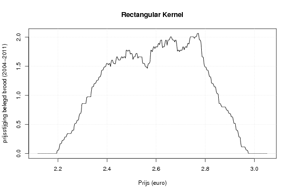
| Title produced by software | Kernel Density Estimation | ||||||||||||||||||||||||||||||||
| Date of computation | Wed, 15 Feb 2012 08:03:15 -0500 | ||||||||||||||||||||||||||||||||
| Cite this page as follows | Statistical Computations at FreeStatistics.org, Office for Research Development and Education, URL https://freestatistics.org/blog/index.php?v=date/2012/Feb/15/t1329311050a55gf14rdt005g1.htm/, Retrieved Tue, 07 May 2024 22:06:44 +0000 | ||||||||||||||||||||||||||||||||
| Statistical Computations at FreeStatistics.org, Office for Research Development and Education, URL https://freestatistics.org/blog/index.php?pk=162428, Retrieved Tue, 07 May 2024 22:06:44 +0000 | |||||||||||||||||||||||||||||||||
| QR Codes: | |||||||||||||||||||||||||||||||||
|
| |||||||||||||||||||||||||||||||||
| Original text written by user: | |||||||||||||||||||||||||||||||||
| IsPrivate? | No (this computation is public) | ||||||||||||||||||||||||||||||||
| User-defined keywords | KDG2011W2EC | ||||||||||||||||||||||||||||||||
| Estimated Impact | 104 | ||||||||||||||||||||||||||||||||
Tree of Dependent Computations | |||||||||||||||||||||||||||||||||
| Family? (F = Feedback message, R = changed R code, M = changed R Module, P = changed Parameters, D = changed Data) | |||||||||||||||||||||||||||||||||
| - [Kernel Density Estimation] [dichtheidsgrafiek...] [2012-02-15 13:03:15] [4080e77d9380e2af46712fd05e0afa1e] [Current] - RMPD [Quartiles] [jens vanpachtenbe...] [2012-05-25 14:27:42] [6c12ae1bbd1f05ed2de376c80d275927] - RMPD [Notched Boxplots] [jens vanpachtenbe...] [2012-05-25 14:32:20] [6c12ae1bbd1f05ed2de376c80d275927] - RMPD [Harrell-Davis Quantiles] [jens vanpachtenbe...] [2012-05-25 14:38:16] [6c12ae1bbd1f05ed2de376c80d275927] - RMPD [Harrell-Davis Quantiles] [jens vanpachtenbe...] [2012-05-25 14:40:42] [6c12ae1bbd1f05ed2de376c80d275927] - RMPD [Mean versus Median] [jens vanpachtenbe...] [2012-05-25 14:52:19] [6c12ae1bbd1f05ed2de376c80d275927] - RMPD [Central Tendency] [jens vanpachtenbe...] [2012-05-25 14:54:42] [6c12ae1bbd1f05ed2de376c80d275927] - RMPD [Mean versus Median] [jens vanpachtenbe...] [2012-05-25 14:59:15] [6c12ae1bbd1f05ed2de376c80d275927] | |||||||||||||||||||||||||||||||||
| Feedback Forum | |||||||||||||||||||||||||||||||||
Post a new message | |||||||||||||||||||||||||||||||||
Dataset | |||||||||||||||||||||||||||||||||
| Dataseries X: | |||||||||||||||||||||||||||||||||
2,3 2,31 2,31 2,32 2,33 2,34 2,36 2,37 2,37 2,38 2,39 2,4 2,4 2,39 2,4 2,42 2,42 2,44 2,44 2,44 2,45 2,46 2,47 2,48 2,48 2,49 2,5 2,51 2,52 2,52 2,52 2,54 2,54 2,54 2,56 2,57 2,58 2,58 2,58 2,58 2,59 2,6 2,61 2,61 2,62 2,63 2,65 2,67 2,68 2,67 2,68 2,68 2,68 2,68 2,69 2,69 2,69 2,7 2,71 2,72 2,71 2,72 2,73 2,74 2,74 2,75 2,75 2,76 2,75 2,78 2,79 2,8 2,81 2,81 2,82 2,82 2,83 2,83 2,84 2,84 2,84 2,86 2,87 | |||||||||||||||||||||||||||||||||
Tables (Output of Computation) | |||||||||||||||||||||||||||||||||
| |||||||||||||||||||||||||||||||||
Figures (Output of Computation) | |||||||||||||||||||||||||||||||||
Input Parameters & R Code | |||||||||||||||||||||||||||||||||
| Parameters (Session): | |||||||||||||||||||||||||||||||||
| par1 = 0 ; | |||||||||||||||||||||||||||||||||
| Parameters (R input): | |||||||||||||||||||||||||||||||||
| par1 = 0 ; | |||||||||||||||||||||||||||||||||
| R code (references can be found in the software module): | |||||||||||||||||||||||||||||||||
if (par1 == '0') bw <- 'nrd0' | |||||||||||||||||||||||||||||||||