Repository of Reproducible Computations

Free Statistics

of Irreproducible Research!

Author's title

Author

*Unverified author*

R Software Module

rwasp_exponentialsmoothing.wasp

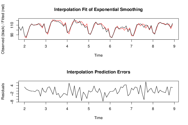
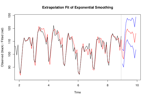
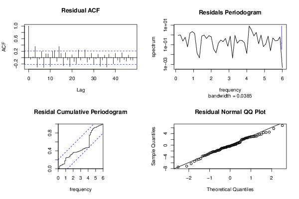
Title produced by software

Exponential Smoothing

Date of computation

Thu, 15 May 2014 09:45:48 -0400

Cite this page as follows

Statistical Computations at FreeStatistics.org, Office for Research Development and Education, URL https://freestatistics.org/blog/index.php?v=date/2014/May/15/t1400161586qn2vh869035gk7v.htm/, Retrieved Tue, 14 May 2024 11:50:15 +0000

Statistical Computations at FreeStatistics.org, Office for Research Development and Education, URL https://freestatistics.org/blog/index.php?pk=234881, Retrieved Tue, 14 May 2024 11:50:15 +0000

QR Codes:

Paste this QR Code to cite your computation.

Original text written by user:

IsPrivate?

No (this computation is public)

User-defined keywords

Estimated Impact

151

Family? (F = Feedback message, R = changed R code, M = changed R Module, P = changed Parameters, D = changed Data)

-       [Exponential Smoothing] [] [2014-05-15 13:45:48] [89aa3cf34f31456ae4e73c425f5126f1] [Current]

Feedback Forum

Post a new message

Dataseries X:

Download CSV

Histogram

Boxplots

Summary of computational transaction
Raw Input	view raw input (R code)
Raw Output	view raw output of R engine
Computing time	2 seconds
R Server	'Gwilym Jenkins' @ jenkins.wessa.net

\begin{tabular}{lllllllll}
\hline
Summary of computational transaction \tabularnewline
Raw Input & view raw input (R code)  \tabularnewline
Raw Output & view raw output of R engine  \tabularnewline
Computing time & 2 seconds \tabularnewline
R Server & 'Gwilym Jenkins' @ jenkins.wessa.net \tabularnewline
\hline
\end{tabular}
%Source: https://freestatistics.org/blog/index.php?pk=234881&T=0

[TABLE]
[ROW][C]Summary of computational transaction[/C][/ROW]
[ROW][C]Raw Input[/C][C]view raw input (R code) [/C][/ROW]
[ROW][C]Raw Output[/C][C]view raw output of R engine [/C][/ROW]
[ROW][C]Computing time[/C][C]2 seconds[/C][/ROW]
[ROW][C]R Server[/C][C]'Gwilym Jenkins' @ jenkins.wessa.net[/C][/ROW]
[/TABLE]
Source: https://freestatistics.org/blog/index.php?pk=234881&T=0

Globally Unique Identifier (entire table): ba.freestatistics.org/blog/index.php?pk=234881&T=0

As an alternative you can also use a QR Code:

The GUIDs for individual cells are displayed in the table below:

Summary of computational transaction
Raw Input	view raw input (R code)
Raw Output	view raw output of R engine
Computing time	2 seconds
R Server	'Gwilym Jenkins' @ jenkins.wessa.net

Estimated Parameters of Exponential Smoothing
Parameter	Value
alpha	0.481112743290017
beta	0.0427927171249243
gamma	0.669608235245175

\begin{tabular}{lllllllll}
\hline
Estimated Parameters of Exponential Smoothing \tabularnewline
Parameter & Value \tabularnewline
alpha & 0.481112743290017 \tabularnewline
beta & 0.0427927171249243 \tabularnewline
gamma & 0.669608235245175 \tabularnewline
\hline
\end{tabular}
%Source: https://freestatistics.org/blog/index.php?pk=234881&T=1

[TABLE]
[ROW][C]Estimated Parameters of Exponential Smoothing[/C][/ROW]
[ROW][C]Parameter[/C][C]Value[/C][/ROW]
[ROW][C]alpha[/C][C]0.481112743290017[/C][/ROW]
[ROW][C]beta[/C][C]0.0427927171249243[/C][/ROW]
[ROW][C]gamma[/C][C]0.669608235245175[/C][/ROW]
[/TABLE]
Source: https://freestatistics.org/blog/index.php?pk=234881&T=1

Globally Unique Identifier (entire table): ba.freestatistics.org/blog/index.php?pk=234881&T=1

As an alternative you can also use a QR Code:

The GUIDs for individual cells are displayed in the table below:

Estimated Parameters of Exponential Smoothing
Parameter	Value
alpha	0.481112743290017
beta	0.0427927171249243
gamma	0.669608235245175

Interpolation Forecasts of Exponential Smoothing
t	Observed	Fitted	Residuals
13	89.6	86.669204059829	2.93079594017095
14	85.3	83.8267518360352	1.47324816396475
15	96.3	95.5508862153964	0.749113784603608
16	107.7	107.492053162629	0.20794683737121
17	112.7	112.76463903006	-0.0646390300596806
18	110.1	110.196416233489	-0.0964162334891085
19	110.4	110.87341999027	-0.47341999027006
20	111.6	110.796795607102	0.803204392898323
21	113.3	112.98007461939	0.319925380609519
22	109	112.766595269585	-3.76659526958532
23	106.5	104.259491638094	2.24050836190645
24	113	113.363609972417	-0.363609972417464
25	95.6	96.5173429199326	-0.917342919932594
26	93.8	91.3193796522052	2.48062034779481
27	106.4	103.29961647735	3.10038352265003
28	116.6	116.255432586731	0.344567413268607
29	119.1	121.573303256676	-2.47330325667642
30	120.9	117.859875691532	3.04012430846832
31	117.3	120.004169462492	-2.70416946249202
32	117.6	119.341191578445	-1.74119157844483
33	115.3	120.123352916874	-4.82335291687438
34	112.3	115.900559489307	-3.60055948930656
35	107.7	109.448980475556	-1.74898047555585
36	113.4	115.535232262471	-2.13523226247095
37	94.3	97.4140769690695	-3.11407696906949
38	97.8	92.0644936622402	5.73550633775979
39	106.6	105.617677407736	0.982322592263884
40	113	116.344991302868	-3.34499130286829
41	122.4	118.580770134244	3.81922986575627
42	114.6	119.612033160258	-5.0120331602584
43	115	115.522316718652	-0.522316718652007
44	118.7	115.924411052547	2.77558894745252
45	110.4	117.582511748763	-7.18251174876296
46	111.6	112.374746597522	-0.774746597522068
47	105.1	107.709402303237	-2.60940230323722
48	107.5	113.013142889264	-5.51314288926439
49	92.9	92.6228385087786	0.277161491221392
50	91	91.7455481447792	-0.745548144779207
51	100.2	100.161608688408	0.0383913115923349
52	112.2	108.544315125481	3.655684874519
53	116.5	116.394616580095	0.105383419905067
54	111.2	112.251397872866	-1.05139787286625
55	113.3	111.389422736856	1.91057726314422
56	112.2	113.920235222147	-1.72023522214747
57	102.2	109.675183842002	-7.47518384200224
58	105.3	106.266770476323	-0.966770476322836
59	96	100.58140884028	-4.58140884027956
60	101.3	103.596705031134	-2.29670503113373
61	86.2	86.5011595701778	-0.301159570177845
62	84.4	84.7138249463801	-0.313824946380095
63	93.4	93.3423971240161	0.0576028759838749
64	104.8	102.723998349651	2.07600165034897
65	106.2	108.281033876226	-2.08103387622621
66	101.9	102.339258927345	-0.439258927345193
67	105.5	102.468818193728	3.03118180627153
68	106.4	103.968193662263	2.43180633773726
69	103.9	99.4976173738507	4.40238262614928
70	108.6	104.085983959579	4.51401604042111
71	96.4	99.9154027519165	-3.51540275191653
72	102.2	104.393152711911	-2.19315271191097
73	90.3	88.1986757853075	2.1013242146925
74	88.5	87.7701623224945	0.729837677505543
75	100.2	97.2587501728194	2.94124982718061
76	111.6	109.017217853465	2.5827821465347
77	111.5	113.672350816431	-2.17235081643112
78	112.9	108.553844505084	4.34615549491583
79	110.7	112.586824791979	-1.88682479197878
80	105.5	111.805866814158	-6.30586681415841
81	110.7	103.930307319738	6.76969268026195
82	108.9	109.859286205331	-0.959286205330585
83	101.3	100.315795595353	0.984204404646505
84	109.6	107.560616786303	2.03938321369698
85	94.4	95.1245634218268	-0.724563421826815
86	91.4	93.0317505869899	-1.63175058698994
87	105.8	102.275681121173	3.52431887882652
88	112.9	114.325300161428	-1.42530016142764
89	116.1	115.452577631331	0.647422368668927
90	113.7	114.066277218644	-0.36627721864447
91	112.9	113.680083955279	-0.780083955279025
92	110.7	111.93267168348	-1.23267168347995
93	114.3	111.181937104546	3.11806289545403
94	109.7	112.734374843189	-3.0343748431893
95	105.7	102.890825887555	2.80917411244458
96	114	111.440884216981	2.55911578301921

\begin{tabular}{lllllllll}
\hline
Interpolation Forecasts of Exponential Smoothing \tabularnewline
t & Observed & Fitted & Residuals \tabularnewline
13 & 89.6 & 86.669204059829 & 2.93079594017095 \tabularnewline
14 & 85.3 & 83.8267518360352 & 1.47324816396475 \tabularnewline
15 & 96.3 & 95.5508862153964 & 0.749113784603608 \tabularnewline
16 & 107.7 & 107.492053162629 & 0.20794683737121 \tabularnewline
17 & 112.7 & 112.76463903006 & -0.0646390300596806 \tabularnewline
18 & 110.1 & 110.196416233489 & -0.0964162334891085 \tabularnewline
19 & 110.4 & 110.87341999027 & -0.47341999027006 \tabularnewline
20 & 111.6 & 110.796795607102 & 0.803204392898323 \tabularnewline
21 & 113.3 & 112.98007461939 & 0.319925380609519 \tabularnewline
22 & 109 & 112.766595269585 & -3.76659526958532 \tabularnewline
23 & 106.5 & 104.259491638094 & 2.24050836190645 \tabularnewline
24 & 113 & 113.363609972417 & -0.363609972417464 \tabularnewline
25 & 95.6 & 96.5173429199326 & -0.917342919932594 \tabularnewline
26 & 93.8 & 91.3193796522052 & 2.48062034779481 \tabularnewline
27 & 106.4 & 103.29961647735 & 3.10038352265003 \tabularnewline
28 & 116.6 & 116.255432586731 & 0.344567413268607 \tabularnewline
29 & 119.1 & 121.573303256676 & -2.47330325667642 \tabularnewline
30 & 120.9 & 117.859875691532 & 3.04012430846832 \tabularnewline
31 & 117.3 & 120.004169462492 & -2.70416946249202 \tabularnewline
32 & 117.6 & 119.341191578445 & -1.74119157844483 \tabularnewline
33 & 115.3 & 120.123352916874 & -4.82335291687438 \tabularnewline
34 & 112.3 & 115.900559489307 & -3.60055948930656 \tabularnewline
35 & 107.7 & 109.448980475556 & -1.74898047555585 \tabularnewline
36 & 113.4 & 115.535232262471 & -2.13523226247095 \tabularnewline
37 & 94.3 & 97.4140769690695 & -3.11407696906949 \tabularnewline
38 & 97.8 & 92.0644936622402 & 5.73550633775979 \tabularnewline
39 & 106.6 & 105.617677407736 & 0.982322592263884 \tabularnewline
40 & 113 & 116.344991302868 & -3.34499130286829 \tabularnewline
41 & 122.4 & 118.580770134244 & 3.81922986575627 \tabularnewline
42 & 114.6 & 119.612033160258 & -5.0120331602584 \tabularnewline
43 & 115 & 115.522316718652 & -0.522316718652007 \tabularnewline
44 & 118.7 & 115.924411052547 & 2.77558894745252 \tabularnewline
45 & 110.4 & 117.582511748763 & -7.18251174876296 \tabularnewline
46 & 111.6 & 112.374746597522 & -0.774746597522068 \tabularnewline
47 & 105.1 & 107.709402303237 & -2.60940230323722 \tabularnewline
48 & 107.5 & 113.013142889264 & -5.51314288926439 \tabularnewline
49 & 92.9 & 92.6228385087786 & 0.277161491221392 \tabularnewline
50 & 91 & 91.7455481447792 & -0.745548144779207 \tabularnewline
51 & 100.2 & 100.161608688408 & 0.0383913115923349 \tabularnewline
52 & 112.2 & 108.544315125481 & 3.655684874519 \tabularnewline
53 & 116.5 & 116.394616580095 & 0.105383419905067 \tabularnewline
54 & 111.2 & 112.251397872866 & -1.05139787286625 \tabularnewline
55 & 113.3 & 111.389422736856 & 1.91057726314422 \tabularnewline
56 & 112.2 & 113.920235222147 & -1.72023522214747 \tabularnewline
57 & 102.2 & 109.675183842002 & -7.47518384200224 \tabularnewline
58 & 105.3 & 106.266770476323 & -0.966770476322836 \tabularnewline
59 & 96 & 100.58140884028 & -4.58140884027956 \tabularnewline
60 & 101.3 & 103.596705031134 & -2.29670503113373 \tabularnewline
61 & 86.2 & 86.5011595701778 & -0.301159570177845 \tabularnewline
62 & 84.4 & 84.7138249463801 & -0.313824946380095 \tabularnewline
63 & 93.4 & 93.3423971240161 & 0.0576028759838749 \tabularnewline
64 & 104.8 & 102.723998349651 & 2.07600165034897 \tabularnewline
65 & 106.2 & 108.281033876226 & -2.08103387622621 \tabularnewline
66 & 101.9 & 102.339258927345 & -0.439258927345193 \tabularnewline
67 & 105.5 & 102.468818193728 & 3.03118180627153 \tabularnewline
68 & 106.4 & 103.968193662263 & 2.43180633773726 \tabularnewline
69 & 103.9 & 99.4976173738507 & 4.40238262614928 \tabularnewline
70 & 108.6 & 104.085983959579 & 4.51401604042111 \tabularnewline
71 & 96.4 & 99.9154027519165 & -3.51540275191653 \tabularnewline
72 & 102.2 & 104.393152711911 & -2.19315271191097 \tabularnewline
73 & 90.3 & 88.1986757853075 & 2.1013242146925 \tabularnewline
74 & 88.5 & 87.7701623224945 & 0.729837677505543 \tabularnewline
75 & 100.2 & 97.2587501728194 & 2.94124982718061 \tabularnewline
76 & 111.6 & 109.017217853465 & 2.5827821465347 \tabularnewline
77 & 111.5 & 113.672350816431 & -2.17235081643112 \tabularnewline
78 & 112.9 & 108.553844505084 & 4.34615549491583 \tabularnewline
79 & 110.7 & 112.586824791979 & -1.88682479197878 \tabularnewline
80 & 105.5 & 111.805866814158 & -6.30586681415841 \tabularnewline
81 & 110.7 & 103.930307319738 & 6.76969268026195 \tabularnewline
82 & 108.9 & 109.859286205331 & -0.959286205330585 \tabularnewline
83 & 101.3 & 100.315795595353 & 0.984204404646505 \tabularnewline
84 & 109.6 & 107.560616786303 & 2.03938321369698 \tabularnewline
85 & 94.4 & 95.1245634218268 & -0.724563421826815 \tabularnewline
86 & 91.4 & 93.0317505869899 & -1.63175058698994 \tabularnewline
87 & 105.8 & 102.275681121173 & 3.52431887882652 \tabularnewline
88 & 112.9 & 114.325300161428 & -1.42530016142764 \tabularnewline
89 & 116.1 & 115.452577631331 & 0.647422368668927 \tabularnewline
90 & 113.7 & 114.066277218644 & -0.36627721864447 \tabularnewline
91 & 112.9 & 113.680083955279 & -0.780083955279025 \tabularnewline
92 & 110.7 & 111.93267168348 & -1.23267168347995 \tabularnewline
93 & 114.3 & 111.181937104546 & 3.11806289545403 \tabularnewline
94 & 109.7 & 112.734374843189 & -3.0343748431893 \tabularnewline
95 & 105.7 & 102.890825887555 & 2.80917411244458 \tabularnewline
96 & 114 & 111.440884216981 & 2.55911578301921 \tabularnewline
\hline
\end{tabular}
%Source: https://freestatistics.org/blog/index.php?pk=234881&T=2

[TABLE]
[ROW][C]Interpolation Forecasts of Exponential Smoothing[/C][/ROW]
[ROW][C]t[/C][C]Observed[/C][C]Fitted[/C][C]Residuals[/C][/ROW]
[ROW][C]13[/C][C]89.6[/C][C]86.669204059829[/C][C]2.93079594017095[/C][/ROW]
[ROW][C]14[/C][C]85.3[/C][C]83.8267518360352[/C][C]1.47324816396475[/C][/ROW]
[ROW][C]15[/C][C]96.3[/C][C]95.5508862153964[/C][C]0.749113784603608[/C][/ROW]
[ROW][C]16[/C][C]107.7[/C][C]107.492053162629[/C][C]0.20794683737121[/C][/ROW]
[ROW][C]17[/C][C]112.7[/C][C]112.76463903006[/C][C]-0.0646390300596806[/C][/ROW]
[ROW][C]18[/C][C]110.1[/C][C]110.196416233489[/C][C]-0.0964162334891085[/C][/ROW]
[ROW][C]19[/C][C]110.4[/C][C]110.87341999027[/C][C]-0.47341999027006[/C][/ROW]
[ROW][C]20[/C][C]111.6[/C][C]110.796795607102[/C][C]0.803204392898323[/C][/ROW]
[ROW][C]21[/C][C]113.3[/C][C]112.98007461939[/C][C]0.319925380609519[/C][/ROW]
[ROW][C]22[/C][C]109[/C][C]112.766595269585[/C][C]-3.76659526958532[/C][/ROW]
[ROW][C]23[/C][C]106.5[/C][C]104.259491638094[/C][C]2.24050836190645[/C][/ROW]
[ROW][C]24[/C][C]113[/C][C]113.363609972417[/C][C]-0.363609972417464[/C][/ROW]
[ROW][C]25[/C][C]95.6[/C][C]96.5173429199326[/C][C]-0.917342919932594[/C][/ROW]
[ROW][C]26[/C][C]93.8[/C][C]91.3193796522052[/C][C]2.48062034779481[/C][/ROW]
[ROW][C]27[/C][C]106.4[/C][C]103.29961647735[/C][C]3.10038352265003[/C][/ROW]
[ROW][C]28[/C][C]116.6[/C][C]116.255432586731[/C][C]0.344567413268607[/C][/ROW]
[ROW][C]29[/C][C]119.1[/C][C]121.573303256676[/C][C]-2.47330325667642[/C][/ROW]
[ROW][C]30[/C][C]120.9[/C][C]117.859875691532[/C][C]3.04012430846832[/C][/ROW]
[ROW][C]31[/C][C]117.3[/C][C]120.004169462492[/C][C]-2.70416946249202[/C][/ROW]
[ROW][C]32[/C][C]117.6[/C][C]119.341191578445[/C][C]-1.74119157844483[/C][/ROW]
[ROW][C]33[/C][C]115.3[/C][C]120.123352916874[/C][C]-4.82335291687438[/C][/ROW]
[ROW][C]34[/C][C]112.3[/C][C]115.900559489307[/C][C]-3.60055948930656[/C][/ROW]
[ROW][C]35[/C][C]107.7[/C][C]109.448980475556[/C][C]-1.74898047555585[/C][/ROW]
[ROW][C]36[/C][C]113.4[/C][C]115.535232262471[/C][C]-2.13523226247095[/C][/ROW]
[ROW][C]37[/C][C]94.3[/C][C]97.4140769690695[/C][C]-3.11407696906949[/C][/ROW]
[ROW][C]38[/C][C]97.8[/C][C]92.0644936622402[/C][C]5.73550633775979[/C][/ROW]
[ROW][C]39[/C][C]106.6[/C][C]105.617677407736[/C][C]0.982322592263884[/C][/ROW]
[ROW][C]40[/C][C]113[/C][C]116.344991302868[/C][C]-3.34499130286829[/C][/ROW]
[ROW][C]41[/C][C]122.4[/C][C]118.580770134244[/C][C]3.81922986575627[/C][/ROW]
[ROW][C]42[/C][C]114.6[/C][C]119.612033160258[/C][C]-5.0120331602584[/C][/ROW]
[ROW][C]43[/C][C]115[/C][C]115.522316718652[/C][C]-0.522316718652007[/C][/ROW]
[ROW][C]44[/C][C]118.7[/C][C]115.924411052547[/C][C]2.77558894745252[/C][/ROW]
[ROW][C]45[/C][C]110.4[/C][C]117.582511748763[/C][C]-7.18251174876296[/C][/ROW]
[ROW][C]46[/C][C]111.6[/C][C]112.374746597522[/C][C]-0.774746597522068[/C][/ROW]
[ROW][C]47[/C][C]105.1[/C][C]107.709402303237[/C][C]-2.60940230323722[/C][/ROW]
[ROW][C]48[/C][C]107.5[/C][C]113.013142889264[/C][C]-5.51314288926439[/C][/ROW]
[ROW][C]49[/C][C]92.9[/C][C]92.6228385087786[/C][C]0.277161491221392[/C][/ROW]
[ROW][C]50[/C][C]91[/C][C]91.7455481447792[/C][C]-0.745548144779207[/C][/ROW]
[ROW][C]51[/C][C]100.2[/C][C]100.161608688408[/C][C]0.0383913115923349[/C][/ROW]
[ROW][C]52[/C][C]112.2[/C][C]108.544315125481[/C][C]3.655684874519[/C][/ROW]
[ROW][C]53[/C][C]116.5[/C][C]116.394616580095[/C][C]0.105383419905067[/C][/ROW]
[ROW][C]54[/C][C]111.2[/C][C]112.251397872866[/C][C]-1.05139787286625[/C][/ROW]
[ROW][C]55[/C][C]113.3[/C][C]111.389422736856[/C][C]1.91057726314422[/C][/ROW]
[ROW][C]56[/C][C]112.2[/C][C]113.920235222147[/C][C]-1.72023522214747[/C][/ROW]
[ROW][C]57[/C][C]102.2[/C][C]109.675183842002[/C][C]-7.47518384200224[/C][/ROW]
[ROW][C]58[/C][C]105.3[/C][C]106.266770476323[/C][C]-0.966770476322836[/C][/ROW]
[ROW][C]59[/C][C]96[/C][C]100.58140884028[/C][C]-4.58140884027956[/C][/ROW]
[ROW][C]60[/C][C]101.3[/C][C]103.596705031134[/C][C]-2.29670503113373[/C][/ROW]
[ROW][C]61[/C][C]86.2[/C][C]86.5011595701778[/C][C]-0.301159570177845[/C][/ROW]
[ROW][C]62[/C][C]84.4[/C][C]84.7138249463801[/C][C]-0.313824946380095[/C][/ROW]
[ROW][C]63[/C][C]93.4[/C][C]93.3423971240161[/C][C]0.0576028759838749[/C][/ROW]
[ROW][C]64[/C][C]104.8[/C][C]102.723998349651[/C][C]2.07600165034897[/C][/ROW]
[ROW][C]65[/C][C]106.2[/C][C]108.281033876226[/C][C]-2.08103387622621[/C][/ROW]
[ROW][C]66[/C][C]101.9[/C][C]102.339258927345[/C][C]-0.439258927345193[/C][/ROW]
[ROW][C]67[/C][C]105.5[/C][C]102.468818193728[/C][C]3.03118180627153[/C][/ROW]
[ROW][C]68[/C][C]106.4[/C][C]103.968193662263[/C][C]2.43180633773726[/C][/ROW]
[ROW][C]69[/C][C]103.9[/C][C]99.4976173738507[/C][C]4.40238262614928[/C][/ROW]
[ROW][C]70[/C][C]108.6[/C][C]104.085983959579[/C][C]4.51401604042111[/C][/ROW]
[ROW][C]71[/C][C]96.4[/C][C]99.9154027519165[/C][C]-3.51540275191653[/C][/ROW]
[ROW][C]72[/C][C]102.2[/C][C]104.393152711911[/C][C]-2.19315271191097[/C][/ROW]
[ROW][C]73[/C][C]90.3[/C][C]88.1986757853075[/C][C]2.1013242146925[/C][/ROW]
[ROW][C]74[/C][C]88.5[/C][C]87.7701623224945[/C][C]0.729837677505543[/C][/ROW]
[ROW][C]75[/C][C]100.2[/C][C]97.2587501728194[/C][C]2.94124982718061[/C][/ROW]
[ROW][C]76[/C][C]111.6[/C][C]109.017217853465[/C][C]2.5827821465347[/C][/ROW]
[ROW][C]77[/C][C]111.5[/C][C]113.672350816431[/C][C]-2.17235081643112[/C][/ROW]
[ROW][C]78[/C][C]112.9[/C][C]108.553844505084[/C][C]4.34615549491583[/C][/ROW]
[ROW][C]79[/C][C]110.7[/C][C]112.586824791979[/C][C]-1.88682479197878[/C][/ROW]
[ROW][C]80[/C][C]105.5[/C][C]111.805866814158[/C][C]-6.30586681415841[/C][/ROW]
[ROW][C]81[/C][C]110.7[/C][C]103.930307319738[/C][C]6.76969268026195[/C][/ROW]
[ROW][C]82[/C][C]108.9[/C][C]109.859286205331[/C][C]-0.959286205330585[/C][/ROW]
[ROW][C]83[/C][C]101.3[/C][C]100.315795595353[/C][C]0.984204404646505[/C][/ROW]
[ROW][C]84[/C][C]109.6[/C][C]107.560616786303[/C][C]2.03938321369698[/C][/ROW]
[ROW][C]85[/C][C]94.4[/C][C]95.1245634218268[/C][C]-0.724563421826815[/C][/ROW]
[ROW][C]86[/C][C]91.4[/C][C]93.0317505869899[/C][C]-1.63175058698994[/C][/ROW]
[ROW][C]87[/C][C]105.8[/C][C]102.275681121173[/C][C]3.52431887882652[/C][/ROW]
[ROW][C]88[/C][C]112.9[/C][C]114.325300161428[/C][C]-1.42530016142764[/C][/ROW]
[ROW][C]89[/C][C]116.1[/C][C]115.452577631331[/C][C]0.647422368668927[/C][/ROW]
[ROW][C]90[/C][C]113.7[/C][C]114.066277218644[/C][C]-0.36627721864447[/C][/ROW]
[ROW][C]91[/C][C]112.9[/C][C]113.680083955279[/C][C]-0.780083955279025[/C][/ROW]
[ROW][C]92[/C][C]110.7[/C][C]111.93267168348[/C][C]-1.23267168347995[/C][/ROW]
[ROW][C]93[/C][C]114.3[/C][C]111.181937104546[/C][C]3.11806289545403[/C][/ROW]
[ROW][C]94[/C][C]109.7[/C][C]112.734374843189[/C][C]-3.0343748431893[/C][/ROW]
[ROW][C]95[/C][C]105.7[/C][C]102.890825887555[/C][C]2.80917411244458[/C][/ROW]
[ROW][C]96[/C][C]114[/C][C]111.440884216981[/C][C]2.55911578301921[/C][/ROW]
[/TABLE]
Source: https://freestatistics.org/blog/index.php?pk=234881&T=2

Globally Unique Identifier (entire table): ba.freestatistics.org/blog/index.php?pk=234881&T=2

As an alternative you can also use a QR Code:

The GUIDs for individual cells are displayed in the table below:

Interpolation Forecasts of Exponential Smoothing
t	Observed	Fitted	Residuals
13	89.6	86.669204059829	2.93079594017095
14	85.3	83.8267518360352	1.47324816396475
15	96.3	95.5508862153964	0.749113784603608
16	107.7	107.492053162629	0.20794683737121
17	112.7	112.76463903006	-0.0646390300596806
18	110.1	110.196416233489	-0.0964162334891085
19	110.4	110.87341999027	-0.47341999027006
20	111.6	110.796795607102	0.803204392898323
21	113.3	112.98007461939	0.319925380609519
22	109	112.766595269585	-3.76659526958532
23	106.5	104.259491638094	2.24050836190645
24	113	113.363609972417	-0.363609972417464
25	95.6	96.5173429199326	-0.917342919932594
26	93.8	91.3193796522052	2.48062034779481
27	106.4	103.29961647735	3.10038352265003
28	116.6	116.255432586731	0.344567413268607
29	119.1	121.573303256676	-2.47330325667642
30	120.9	117.859875691532	3.04012430846832
31	117.3	120.004169462492	-2.70416946249202
32	117.6	119.341191578445	-1.74119157844483
33	115.3	120.123352916874	-4.82335291687438
34	112.3	115.900559489307	-3.60055948930656
35	107.7	109.448980475556	-1.74898047555585
36	113.4	115.535232262471	-2.13523226247095
37	94.3	97.4140769690695	-3.11407696906949
38	97.8	92.0644936622402	5.73550633775979
39	106.6	105.617677407736	0.982322592263884
40	113	116.344991302868	-3.34499130286829
41	122.4	118.580770134244	3.81922986575627
42	114.6	119.612033160258	-5.0120331602584
43	115	115.522316718652	-0.522316718652007
44	118.7	115.924411052547	2.77558894745252
45	110.4	117.582511748763	-7.18251174876296
46	111.6	112.374746597522	-0.774746597522068
47	105.1	107.709402303237	-2.60940230323722
48	107.5	113.013142889264	-5.51314288926439
49	92.9	92.6228385087786	0.277161491221392
50	91	91.7455481447792	-0.745548144779207
51	100.2	100.161608688408	0.0383913115923349
52	112.2	108.544315125481	3.655684874519
53	116.5	116.394616580095	0.105383419905067
54	111.2	112.251397872866	-1.05139787286625
55	113.3	111.389422736856	1.91057726314422
56	112.2	113.920235222147	-1.72023522214747
57	102.2	109.675183842002	-7.47518384200224
58	105.3	106.266770476323	-0.966770476322836
59	96	100.58140884028	-4.58140884027956
60	101.3	103.596705031134	-2.29670503113373
61	86.2	86.5011595701778	-0.301159570177845
62	84.4	84.7138249463801	-0.313824946380095
63	93.4	93.3423971240161	0.0576028759838749
64	104.8	102.723998349651	2.07600165034897
65	106.2	108.281033876226	-2.08103387622621
66	101.9	102.339258927345	-0.439258927345193
67	105.5	102.468818193728	3.03118180627153
68	106.4	103.968193662263	2.43180633773726
69	103.9	99.4976173738507	4.40238262614928
70	108.6	104.085983959579	4.51401604042111
71	96.4	99.9154027519165	-3.51540275191653
72	102.2	104.393152711911	-2.19315271191097
73	90.3	88.1986757853075	2.1013242146925
74	88.5	87.7701623224945	0.729837677505543
75	100.2	97.2587501728194	2.94124982718061
76	111.6	109.017217853465	2.5827821465347
77	111.5	113.672350816431	-2.17235081643112
78	112.9	108.553844505084	4.34615549491583
79	110.7	112.586824791979	-1.88682479197878
80	105.5	111.805866814158	-6.30586681415841
81	110.7	103.930307319738	6.76969268026195
82	108.9	109.859286205331	-0.959286205330585
83	101.3	100.315795595353	0.984204404646505
84	109.6	107.560616786303	2.03938321369698
85	94.4	95.1245634218268	-0.724563421826815
86	91.4	93.0317505869899	-1.63175058698994
87	105.8	102.275681121173	3.52431887882652
88	112.9	114.325300161428	-1.42530016142764
89	116.1	115.452577631331	0.647422368668927
90	113.7	114.066277218644	-0.36627721864447
91	112.9	113.680083955279	-0.780083955279025
92	110.7	111.93267168348	-1.23267168347995
93	114.3	111.181937104546	3.11806289545403
94	109.7	112.734374843189	-3.0343748431893
95	105.7	102.890825887555	2.80917411244458
96	114	111.440884216981	2.55911578301921

Extrapolation Forecasts of Exponential Smoothing
t	Forecast	95% Lower Bound	95% Upper Bound
97	98.365842444678	92.7288962626415	104.002788626714
98	96.392638604587	90.0860476076028	102.699229601571
99	108.332917791249	101.372967892587	115.29286768991
100	117.014442254563	109.411446979761	124.617437529366
101	119.624215061947	111.384437710755	127.86399241314
102	117.637486546336	108.764323600626	126.510649492047
103	117.354543408257	107.849295180884	126.859791635631
104	115.912054917982	105.774449799938	126.049660036025
105	117.378288243257	106.60685199822	128.149724488294
106	115.340965361504	103.933288790784	126.748641932224
107	109.09816379714	97.0511013943494	121.145226199931
108	116.262496988003	103.572317348288	128.952676627718

\begin{tabular}{lllllllll}
\hline
Extrapolation Forecasts of Exponential Smoothing \tabularnewline
t & Forecast & 95% Lower Bound & 95% Upper Bound \tabularnewline
97 & 98.365842444678 & 92.7288962626415 & 104.002788626714 \tabularnewline
98 & 96.392638604587 & 90.0860476076028 & 102.699229601571 \tabularnewline
99 & 108.332917791249 & 101.372967892587 & 115.29286768991 \tabularnewline
100 & 117.014442254563 & 109.411446979761 & 124.617437529366 \tabularnewline
101 & 119.624215061947 & 111.384437710755 & 127.86399241314 \tabularnewline
102 & 117.637486546336 & 108.764323600626 & 126.510649492047 \tabularnewline
103 & 117.354543408257 & 107.849295180884 & 126.859791635631 \tabularnewline
104 & 115.912054917982 & 105.774449799938 & 126.049660036025 \tabularnewline
105 & 117.378288243257 & 106.60685199822 & 128.149724488294 \tabularnewline
106 & 115.340965361504 & 103.933288790784 & 126.748641932224 \tabularnewline
107 & 109.09816379714 & 97.0511013943494 & 121.145226199931 \tabularnewline
108 & 116.262496988003 & 103.572317348288 & 128.952676627718 \tabularnewline
\hline
\end{tabular}
%Source: https://freestatistics.org/blog/index.php?pk=234881&T=3

[TABLE]
[ROW][C]Extrapolation Forecasts of Exponential Smoothing[/C][/ROW]
[ROW][C]t[/C][C]Forecast[/C][C]95% Lower Bound[/C][C]95% Upper Bound[/C][/ROW]
[ROW][C]97[/C][C]98.365842444678[/C][C]92.7288962626415[/C][C]104.002788626714[/C][/ROW]
[ROW][C]98[/C][C]96.392638604587[/C][C]90.0860476076028[/C][C]102.699229601571[/C][/ROW]
[ROW][C]99[/C][C]108.332917791249[/C][C]101.372967892587[/C][C]115.29286768991[/C][/ROW]
[ROW][C]100[/C][C]117.014442254563[/C][C]109.411446979761[/C][C]124.617437529366[/C][/ROW]
[ROW][C]101[/C][C]119.624215061947[/C][C]111.384437710755[/C][C]127.86399241314[/C][/ROW]
[ROW][C]102[/C][C]117.637486546336[/C][C]108.764323600626[/C][C]126.510649492047[/C][/ROW]
[ROW][C]103[/C][C]117.354543408257[/C][C]107.849295180884[/C][C]126.859791635631[/C][/ROW]
[ROW][C]104[/C][C]115.912054917982[/C][C]105.774449799938[/C][C]126.049660036025[/C][/ROW]
[ROW][C]105[/C][C]117.378288243257[/C][C]106.60685199822[/C][C]128.149724488294[/C][/ROW]
[ROW][C]106[/C][C]115.340965361504[/C][C]103.933288790784[/C][C]126.748641932224[/C][/ROW]
[ROW][C]107[/C][C]109.09816379714[/C][C]97.0511013943494[/C][C]121.145226199931[/C][/ROW]
[ROW][C]108[/C][C]116.262496988003[/C][C]103.572317348288[/C][C]128.952676627718[/C][/ROW]
[/TABLE]
Source: https://freestatistics.org/blog/index.php?pk=234881&T=3

Globally Unique Identifier (entire table): ba.freestatistics.org/blog/index.php?pk=234881&T=3

As an alternative you can also use a QR Code:

The GUIDs for individual cells are displayed in the table below:

Extrapolation Forecasts of Exponential Smoothing
t	Forecast	95% Lower Bound	95% Upper Bound
97	98.365842444678	92.7288962626415	104.002788626714
98	96.392638604587	90.0860476076028	102.699229601571
99	108.332917791249	101.372967892587	115.29286768991
100	117.014442254563	109.411446979761	124.617437529366
101	119.624215061947	111.384437710755	127.86399241314
102	117.637486546336	108.764323600626	126.510649492047
103	117.354543408257	107.849295180884	126.859791635631
104	115.912054917982	105.774449799938	126.049660036025
105	117.378288243257	106.60685199822	128.149724488294
106	115.340965361504	103.933288790784	126.748641932224
107	109.09816379714	97.0511013943494	121.145226199931
108	116.262496988003	103.572317348288	128.952676627718

Figure 1

PNG link

Postscript link

PDF link

Figure 2

PNG link

Postscript link

PDF link

Figure 3

PNG link

Postscript link

PDF link

Parameters (Session):

par1 = 12 ; par2 = Triple ; par3 = additive ;

Parameters (R input):

par1 = 12 ; par2 = Triple ; par3 = additive ;

R code (references can be found in the software module):

par1 <- as.numeric(par1)
if (par2 == 'Single') K <- 1
if (par2 == 'Double') K <- 2
if (par2 == 'Triple') K <- par1
nx <- length(x)
nxmK <- nx - K
x <- ts(x, frequency = par1)
if (par2 == 'Single') fit <- HoltWinters(x, gamma=F, beta=F)
if (par2 == 'Double') fit <- HoltWinters(x, gamma=F)
if (par2 == 'Triple') fit <- HoltWinters(x, seasonal=par3)
fit
myresid <- x - fit$fitted[,'xhat']
bitmap(file='test1.png')
op <- par(mfrow=c(2,1))
plot(fit,ylab='Observed (black) / Fitted (red)',main='Interpolation Fit of Exponential Smoothing')
plot(myresid,ylab='Residuals',main='Interpolation Prediction Errors')
par(op)
dev.off()
bitmap(file='test2.png')
p <- predict(fit, par1, prediction.interval=TRUE)
np <- length(p[,1])
plot(fit,p,ylab='Observed (black) / Fitted (red)',main='Extrapolation Fit of Exponential Smoothing')
dev.off()
bitmap(file='test3.png')
op <- par(mfrow = c(2,2))
acf(as.numeric(myresid),lag.max = nx/2,main='Residual ACF')
spectrum(myresid,main='Residals Periodogram')
cpgram(myresid,main='Residal Cumulative Periodogram')
qqnorm(myresid,main='Residual Normal QQ Plot')
qqline(myresid)
par(op)
dev.off()
load(file='createtable')
a<-table.start()
a<-table.row.start(a)
a<-table.element(a,'Estimated Parameters of Exponential Smoothing',2,TRUE)
a<-table.row.end(a)
a<-table.row.start(a)
a<-table.element(a,'Parameter',header=TRUE)
a<-table.element(a,'Value',header=TRUE)
a<-table.row.end(a)
a<-table.row.start(a)
a<-table.element(a,'alpha',header=TRUE)
a<-table.element(a,fit$alpha)
a<-table.row.end(a)
a<-table.row.start(a)
a<-table.element(a,'beta',header=TRUE)
a<-table.element(a,fit$beta)
a<-table.row.end(a)
a<-table.row.start(a)
a<-table.element(a,'gamma',header=TRUE)
a<-table.element(a,fit$gamma)
a<-table.row.end(a)
a<-table.end(a)
table.save(a,file='mytable.tab')
a<-table.start()
a<-table.row.start(a)
a<-table.element(a,'Interpolation Forecasts of Exponential Smoothing',4,TRUE)
a<-table.row.end(a)
a<-table.row.start(a)
a<-table.element(a,'t',header=TRUE)
a<-table.element(a,'Observed',header=TRUE)
a<-table.element(a,'Fitted',header=TRUE)
a<-table.element(a,'Residuals',header=TRUE)
a<-table.row.end(a)
for (i in 1:nxmK) {
a<-table.row.start(a)
a<-table.element(a,i+K,header=TRUE)
a<-table.element(a,x[i+K])
a<-table.element(a,fit$fitted[i,'xhat'])
a<-table.element(a,myresid[i])
a<-table.row.end(a)
}
a<-table.end(a)
table.save(a,file='mytable1.tab')
a<-table.start()
a<-table.row.start(a)
a<-table.element(a,'Extrapolation Forecasts of Exponential Smoothing',4,TRUE)
a<-table.row.end(a)
a<-table.row.start(a)
a<-table.element(a,'t',header=TRUE)
a<-table.element(a,'Forecast',header=TRUE)
a<-table.element(a,'95% Lower Bound',header=TRUE)
a<-table.element(a,'95% Upper Bound',header=TRUE)
a<-table.row.end(a)
for (i in 1:np) {
a<-table.row.start(a)
a<-table.element(a,nx+i,header=TRUE)
a<-table.element(a,p[i,'fit'])
a<-table.element(a,p[i,'lwr'])
a<-table.element(a,p[i,'upr'])
a<-table.row.end(a)
}
a<-table.end(a)
table.save(a,file='mytable2.tab')

Free Statistics

Description of Statistical Computation

Tree of Dependent Computations

Dataset

Tables (Output of Computation)

Figures (Output of Computation)

Input Parameters & R Code