Repository of Reproducible Computations

Free Statistics

of Irreproducible Research!

Author's title

Author

*Unverified author*

R Software Module

rwasp_decompose.wasp

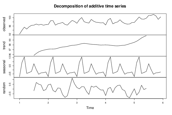
Title produced by software

Classical Decomposition

Date of computation

Sat, 26 Nov 2016 17:44:30 +0000

Cite this page as follows

Statistical Computations at FreeStatistics.org, Office for Research Development and Education, URL https://freestatistics.org/blog/index.php?v=date/2016/Nov/26/t148018230222nbz1y4vff2v29.htm/, Retrieved Fri, 03 May 2024 23:23:49 +0200

Statistical Computations at FreeStatistics.org, Office for Research Development and Education, URL https://freestatistics.org/blog/index.php?pk=, Retrieved Fri, 03 May 2024 23:23:49 +0200

QR Codes:

Paste this QR Code to cite your computation.

Original text written by user:

IsPrivate?

No (this computation is public)

User-defined keywords

Estimated Impact

Dataseries X:

Download CSV

Histogram

Boxplots

Summary of computational transaction
Raw Input	view raw input (R code)
Raw Output	view raw output of R engine
Computing time	1 seconds
R Server	'Gwilym Jenkins' @ jenkins.wessa.net

\begin{tabular}{lllllllll}
\hline
Summary of computational transaction \tabularnewline
Raw Input & view raw input (R code)  \tabularnewline
Raw Output & view raw output of R engine  \tabularnewline
Computing time & 1 seconds \tabularnewline
R Server & 'Gwilym Jenkins' @ jenkins.wessa.net \tabularnewline
\hline
\end{tabular}
%Source: https://freestatistics.org/blog/index.php?pk=&T=0

[TABLE]
[ROW][C]Summary of computational transaction[/C][/ROW]
[ROW][C]Raw Input[/C][C]view raw input (R code) [/C][/ROW]
[ROW][C]Raw Output[/C][C]view raw output of R engine [/C][/ROW]
[ROW][C]Computing time[/C][C]1 seconds[/C][/ROW]
[ROW][C]R Server[/C][C]'Gwilym Jenkins' @ jenkins.wessa.net[/C][/ROW]
[/TABLE]
Source: https://freestatistics.org/blog/index.php?pk=&T=0

Globally Unique Identifier (entire table): ba.freestatistics.org/blog/index.php?pk=&T=0

As an alternative you can also use a QR Code:

The GUIDs for individual cells are displayed in the table below:

Summary of computational transaction
Raw Input	view raw input (R code)
Raw Output	view raw output of R engine
Computing time	1 seconds
R Server	'Gwilym Jenkins' @ jenkins.wessa.net

Classical Decomposition by Moving Averages
t	Observations	Fit	Trend	Seasonal	Random
1	92.1	NA	NA	-0.829271	NA
2	93.91	NA	NA	0.903125	NA
3	95.46	NA	NA	1.59656	NA
4	94.54	NA	NA	-0.436771	NA
5	95.63	NA	NA	-0.329271	NA
6	96.32	NA	NA	-0.1875	NA
7	96.42	96.5976	95.8392	0.758438	-0.177604
8	96.95	96.2673	96.2258	0.0414583	0.682708
9	96.52	96.0105	96.5508	-0.540313	0.509479
10	96.82	96.3917	96.7608	-0.369167	0.428333
11	96.4	96.5555	96.9008	-0.345312	-0.155521
12	96.69	96.743	97.005	-0.261979	-0.0530208
13	96.72	96.2741	97.1033	-0.829271	0.445937
14	98.57	98.0544	97.1512	0.903125	0.515625
15	98.6	98.7378	97.1412	1.59656	-0.137812
16	96.44	96.7366	97.1733	-0.436771	-0.296563
17	97.09	96.9745	97.3038	-0.329271	0.115521
18	97.36	97.275	97.4625	-0.1875	0.085
19	97.74	98.3097	97.5512	0.758438	-0.569688
20	96.78	97.6381	97.5967	0.0414583	-0.858125
21	96.45	97.1384	97.6787	-0.540313	-0.688437
22	97.66	97.4408	97.81	-0.369167	0.219167
23	98.69	97.5584	97.9037	-0.345312	1.13156
24	98.21	97.6697	97.9317	-0.261979	0.540312
25	97.33	97.1661	97.9954	-0.829271	0.163854
26	99.05	99.0231	98.12	0.903125	0.026875
27	100.09	99.8382	98.2417	1.59656	0.251771
28	98.1	97.8645	98.3012	-0.436771	0.235521
29	97.68	97.9249	98.2542	-0.329271	-0.244896
30	97.44	97.9929	98.1804	-0.1875	-0.552917
31	99.19	98.8793	98.1208	0.758438	0.310729
32	98.32	98.1219	98.0804	0.0414583	0.198125
33	97.83	97.518	98.0583	-0.540313	0.311979
34	97.71	97.6292	97.9983	-0.369167	0.0808333
35	97.51	97.6076	97.9529	-0.345312	-0.0976042
36	97.62	97.7109	97.9729	-0.261979	-0.0909375
37	96.49	97.1582	97.9875	-0.829271	-0.668229
38	98.92	98.8652	97.9621	0.903125	0.0547917
39	99.69	99.5157	97.9192	1.59656	0.174271
40	97.06	97.4249	97.8617	-0.436771	-0.364896
41	97.63	97.4774	97.8067	-0.329271	0.152604
42	97.97	97.5992	97.7867	-0.1875	0.370833
43	99.01	98.5993	97.8408	0.758438	0.410729
44	97.89	97.9385	97.8971	0.0414583	-0.0485417
45	97.23	97.3889	97.9292	-0.540313	-0.158854
46	96.93	97.6842	98.0533	-0.369167	-0.754167
47	96.97	97.8743	98.2196	-0.345312	-0.904271
48	97.68	98.1022	98.3642	-0.261979	-0.422187
49	97.73	97.6974	98.5267	-0.829271	0.0326042
50	99.03	99.6531	98.75	0.903125	-0.623125
51	100.35	100.664	99.0675	1.59656	-0.314062
52	99.38	98.9799	99.4167	-0.436771	0.400104
53	99.3	99.3491	99.6783	-0.329271	-0.0490625
54	99.77	99.6987	99.8862	-0.1875	0.07125
55	101.11	NA	NA	0.758438	NA
56	101.15	NA	NA	0.0414583	NA
57	101.59	NA	NA	-0.540313	NA
58	100.95	NA	NA	-0.369167	NA
59	99.23	NA	NA	-0.345312	NA
60	100.41	NA	NA	-0.261979	NA

\begin{tabular}{lllllllll}
\hline
Classical Decomposition by Moving Averages \tabularnewline
t & Observations & Fit & Trend & Seasonal & Random \tabularnewline
1 & 92.1 & NA & NA & -0.829271 & NA \tabularnewline
2 & 93.91 & NA & NA & 0.903125 & NA \tabularnewline
3 & 95.46 & NA & NA & 1.59656 & NA \tabularnewline
4 & 94.54 & NA & NA & -0.436771 & NA \tabularnewline
5 & 95.63 & NA & NA & -0.329271 & NA \tabularnewline
6 & 96.32 & NA & NA & -0.1875 & NA \tabularnewline
7 & 96.42 & 96.5976 & 95.8392 & 0.758438 & -0.177604 \tabularnewline
8 & 96.95 & 96.2673 & 96.2258 & 0.0414583 & 0.682708 \tabularnewline
9 & 96.52 & 96.0105 & 96.5508 & -0.540313 & 0.509479 \tabularnewline
10 & 96.82 & 96.3917 & 96.7608 & -0.369167 & 0.428333 \tabularnewline
11 & 96.4 & 96.5555 & 96.9008 & -0.345312 & -0.155521 \tabularnewline
12 & 96.69 & 96.743 & 97.005 & -0.261979 & -0.0530208 \tabularnewline
13 & 96.72 & 96.2741 & 97.1033 & -0.829271 & 0.445937 \tabularnewline
14 & 98.57 & 98.0544 & 97.1512 & 0.903125 & 0.515625 \tabularnewline
15 & 98.6 & 98.7378 & 97.1412 & 1.59656 & -0.137812 \tabularnewline
16 & 96.44 & 96.7366 & 97.1733 & -0.436771 & -0.296563 \tabularnewline
17 & 97.09 & 96.9745 & 97.3038 & -0.329271 & 0.115521 \tabularnewline
18 & 97.36 & 97.275 & 97.4625 & -0.1875 & 0.085 \tabularnewline
19 & 97.74 & 98.3097 & 97.5512 & 0.758438 & -0.569688 \tabularnewline
20 & 96.78 & 97.6381 & 97.5967 & 0.0414583 & -0.858125 \tabularnewline
21 & 96.45 & 97.1384 & 97.6787 & -0.540313 & -0.688437 \tabularnewline
22 & 97.66 & 97.4408 & 97.81 & -0.369167 & 0.219167 \tabularnewline
23 & 98.69 & 97.5584 & 97.9037 & -0.345312 & 1.13156 \tabularnewline
24 & 98.21 & 97.6697 & 97.9317 & -0.261979 & 0.540312 \tabularnewline
25 & 97.33 & 97.1661 & 97.9954 & -0.829271 & 0.163854 \tabularnewline
26 & 99.05 & 99.0231 & 98.12 & 0.903125 & 0.026875 \tabularnewline
27 & 100.09 & 99.8382 & 98.2417 & 1.59656 & 0.251771 \tabularnewline
28 & 98.1 & 97.8645 & 98.3012 & -0.436771 & 0.235521 \tabularnewline
29 & 97.68 & 97.9249 & 98.2542 & -0.329271 & -0.244896 \tabularnewline
30 & 97.44 & 97.9929 & 98.1804 & -0.1875 & -0.552917 \tabularnewline
31 & 99.19 & 98.8793 & 98.1208 & 0.758438 & 0.310729 \tabularnewline
32 & 98.32 & 98.1219 & 98.0804 & 0.0414583 & 0.198125 \tabularnewline
33 & 97.83 & 97.518 & 98.0583 & -0.540313 & 0.311979 \tabularnewline
34 & 97.71 & 97.6292 & 97.9983 & -0.369167 & 0.0808333 \tabularnewline
35 & 97.51 & 97.6076 & 97.9529 & -0.345312 & -0.0976042 \tabularnewline
36 & 97.62 & 97.7109 & 97.9729 & -0.261979 & -0.0909375 \tabularnewline
37 & 96.49 & 97.1582 & 97.9875 & -0.829271 & -0.668229 \tabularnewline
38 & 98.92 & 98.8652 & 97.9621 & 0.903125 & 0.0547917 \tabularnewline
39 & 99.69 & 99.5157 & 97.9192 & 1.59656 & 0.174271 \tabularnewline
40 & 97.06 & 97.4249 & 97.8617 & -0.436771 & -0.364896 \tabularnewline
41 & 97.63 & 97.4774 & 97.8067 & -0.329271 & 0.152604 \tabularnewline
42 & 97.97 & 97.5992 & 97.7867 & -0.1875 & 0.370833 \tabularnewline
43 & 99.01 & 98.5993 & 97.8408 & 0.758438 & 0.410729 \tabularnewline
44 & 97.89 & 97.9385 & 97.8971 & 0.0414583 & -0.0485417 \tabularnewline
45 & 97.23 & 97.3889 & 97.9292 & -0.540313 & -0.158854 \tabularnewline
46 & 96.93 & 97.6842 & 98.0533 & -0.369167 & -0.754167 \tabularnewline
47 & 96.97 & 97.8743 & 98.2196 & -0.345312 & -0.904271 \tabularnewline
48 & 97.68 & 98.1022 & 98.3642 & -0.261979 & -0.422187 \tabularnewline
49 & 97.73 & 97.6974 & 98.5267 & -0.829271 & 0.0326042 \tabularnewline
50 & 99.03 & 99.6531 & 98.75 & 0.903125 & -0.623125 \tabularnewline
51 & 100.35 & 100.664 & 99.0675 & 1.59656 & -0.314062 \tabularnewline
52 & 99.38 & 98.9799 & 99.4167 & -0.436771 & 0.400104 \tabularnewline
53 & 99.3 & 99.3491 & 99.6783 & -0.329271 & -0.0490625 \tabularnewline
54 & 99.77 & 99.6987 & 99.8862 & -0.1875 & 0.07125 \tabularnewline
55 & 101.11 & NA & NA & 0.758438 & NA \tabularnewline
56 & 101.15 & NA & NA & 0.0414583 & NA \tabularnewline
57 & 101.59 & NA & NA & -0.540313 & NA \tabularnewline
58 & 100.95 & NA & NA & -0.369167 & NA \tabularnewline
59 & 99.23 & NA & NA & -0.345312 & NA \tabularnewline
60 & 100.41 & NA & NA & -0.261979 & NA \tabularnewline
\hline
\end{tabular}
%Source: https://freestatistics.org/blog/index.php?pk=&T=1

[TABLE]
[ROW][C]Classical Decomposition by Moving Averages[/C][/ROW]
[ROW][C]t[/C][C]Observations[/C][C]Fit[/C][C]Trend[/C][C]Seasonal[/C][C]Random[/C][/ROW]
[ROW][C]1[/C][C]92.1[/C][C]NA[/C][C]NA[/C][C]-0.829271[/C][C]NA[/C][/ROW]
[ROW][C]2[/C][C]93.91[/C][C]NA[/C][C]NA[/C][C]0.903125[/C][C]NA[/C][/ROW]
[ROW][C]3[/C][C]95.46[/C][C]NA[/C][C]NA[/C][C]1.59656[/C][C]NA[/C][/ROW]
[ROW][C]4[/C][C]94.54[/C][C]NA[/C][C]NA[/C][C]-0.436771[/C][C]NA[/C][/ROW]
[ROW][C]5[/C][C]95.63[/C][C]NA[/C][C]NA[/C][C]-0.329271[/C][C]NA[/C][/ROW]
[ROW][C]6[/C][C]96.32[/C][C]NA[/C][C]NA[/C][C]-0.1875[/C][C]NA[/C][/ROW]
[ROW][C]7[/C][C]96.42[/C][C]96.5976[/C][C]95.8392[/C][C]0.758438[/C][C]-0.177604[/C][/ROW]
[ROW][C]8[/C][C]96.95[/C][C]96.2673[/C][C]96.2258[/C][C]0.0414583[/C][C]0.682708[/C][/ROW]
[ROW][C]9[/C][C]96.52[/C][C]96.0105[/C][C]96.5508[/C][C]-0.540313[/C][C]0.509479[/C][/ROW]
[ROW][C]10[/C][C]96.82[/C][C]96.3917[/C][C]96.7608[/C][C]-0.369167[/C][C]0.428333[/C][/ROW]
[ROW][C]11[/C][C]96.4[/C][C]96.5555[/C][C]96.9008[/C][C]-0.345312[/C][C]-0.155521[/C][/ROW]
[ROW][C]12[/C][C]96.69[/C][C]96.743[/C][C]97.005[/C][C]-0.261979[/C][C]-0.0530208[/C][/ROW]
[ROW][C]13[/C][C]96.72[/C][C]96.2741[/C][C]97.1033[/C][C]-0.829271[/C][C]0.445937[/C][/ROW]
[ROW][C]14[/C][C]98.57[/C][C]98.0544[/C][C]97.1512[/C][C]0.903125[/C][C]0.515625[/C][/ROW]
[ROW][C]15[/C][C]98.6[/C][C]98.7378[/C][C]97.1412[/C][C]1.59656[/C][C]-0.137812[/C][/ROW]
[ROW][C]16[/C][C]96.44[/C][C]96.7366[/C][C]97.1733[/C][C]-0.436771[/C][C]-0.296563[/C][/ROW]
[ROW][C]17[/C][C]97.09[/C][C]96.9745[/C][C]97.3038[/C][C]-0.329271[/C][C]0.115521[/C][/ROW]
[ROW][C]18[/C][C]97.36[/C][C]97.275[/C][C]97.4625[/C][C]-0.1875[/C][C]0.085[/C][/ROW]
[ROW][C]19[/C][C]97.74[/C][C]98.3097[/C][C]97.5512[/C][C]0.758438[/C][C]-0.569688[/C][/ROW]
[ROW][C]20[/C][C]96.78[/C][C]97.6381[/C][C]97.5967[/C][C]0.0414583[/C][C]-0.858125[/C][/ROW]
[ROW][C]21[/C][C]96.45[/C][C]97.1384[/C][C]97.6787[/C][C]-0.540313[/C][C]-0.688437[/C][/ROW]
[ROW][C]22[/C][C]97.66[/C][C]97.4408[/C][C]97.81[/C][C]-0.369167[/C][C]0.219167[/C][/ROW]
[ROW][C]23[/C][C]98.69[/C][C]97.5584[/C][C]97.9037[/C][C]-0.345312[/C][C]1.13156[/C][/ROW]
[ROW][C]24[/C][C]98.21[/C][C]97.6697[/C][C]97.9317[/C][C]-0.261979[/C][C]0.540312[/C][/ROW]
[ROW][C]25[/C][C]97.33[/C][C]97.1661[/C][C]97.9954[/C][C]-0.829271[/C][C]0.163854[/C][/ROW]
[ROW][C]26[/C][C]99.05[/C][C]99.0231[/C][C]98.12[/C][C]0.903125[/C][C]0.026875[/C][/ROW]
[ROW][C]27[/C][C]100.09[/C][C]99.8382[/C][C]98.2417[/C][C]1.59656[/C][C]0.251771[/C][/ROW]
[ROW][C]28[/C][C]98.1[/C][C]97.8645[/C][C]98.3012[/C][C]-0.436771[/C][C]0.235521[/C][/ROW]
[ROW][C]29[/C][C]97.68[/C][C]97.9249[/C][C]98.2542[/C][C]-0.329271[/C][C]-0.244896[/C][/ROW]
[ROW][C]30[/C][C]97.44[/C][C]97.9929[/C][C]98.1804[/C][C]-0.1875[/C][C]-0.552917[/C][/ROW]
[ROW][C]31[/C][C]99.19[/C][C]98.8793[/C][C]98.1208[/C][C]0.758438[/C][C]0.310729[/C][/ROW]
[ROW][C]32[/C][C]98.32[/C][C]98.1219[/C][C]98.0804[/C][C]0.0414583[/C][C]0.198125[/C][/ROW]
[ROW][C]33[/C][C]97.83[/C][C]97.518[/C][C]98.0583[/C][C]-0.540313[/C][C]0.311979[/C][/ROW]
[ROW][C]34[/C][C]97.71[/C][C]97.6292[/C][C]97.9983[/C][C]-0.369167[/C][C]0.0808333[/C][/ROW]
[ROW][C]35[/C][C]97.51[/C][C]97.6076[/C][C]97.9529[/C][C]-0.345312[/C][C]-0.0976042[/C][/ROW]
[ROW][C]36[/C][C]97.62[/C][C]97.7109[/C][C]97.9729[/C][C]-0.261979[/C][C]-0.0909375[/C][/ROW]
[ROW][C]37[/C][C]96.49[/C][C]97.1582[/C][C]97.9875[/C][C]-0.829271[/C][C]-0.668229[/C][/ROW]
[ROW][C]38[/C][C]98.92[/C][C]98.8652[/C][C]97.9621[/C][C]0.903125[/C][C]0.0547917[/C][/ROW]
[ROW][C]39[/C][C]99.69[/C][C]99.5157[/C][C]97.9192[/C][C]1.59656[/C][C]0.174271[/C][/ROW]
[ROW][C]40[/C][C]97.06[/C][C]97.4249[/C][C]97.8617[/C][C]-0.436771[/C][C]-0.364896[/C][/ROW]
[ROW][C]41[/C][C]97.63[/C][C]97.4774[/C][C]97.8067[/C][C]-0.329271[/C][C]0.152604[/C][/ROW]
[ROW][C]42[/C][C]97.97[/C][C]97.5992[/C][C]97.7867[/C][C]-0.1875[/C][C]0.370833[/C][/ROW]
[ROW][C]43[/C][C]99.01[/C][C]98.5993[/C][C]97.8408[/C][C]0.758438[/C][C]0.410729[/C][/ROW]
[ROW][C]44[/C][C]97.89[/C][C]97.9385[/C][C]97.8971[/C][C]0.0414583[/C][C]-0.0485417[/C][/ROW]
[ROW][C]45[/C][C]97.23[/C][C]97.3889[/C][C]97.9292[/C][C]-0.540313[/C][C]-0.158854[/C][/ROW]
[ROW][C]46[/C][C]96.93[/C][C]97.6842[/C][C]98.0533[/C][C]-0.369167[/C][C]-0.754167[/C][/ROW]
[ROW][C]47[/C][C]96.97[/C][C]97.8743[/C][C]98.2196[/C][C]-0.345312[/C][C]-0.904271[/C][/ROW]
[ROW][C]48[/C][C]97.68[/C][C]98.1022[/C][C]98.3642[/C][C]-0.261979[/C][C]-0.422187[/C][/ROW]
[ROW][C]49[/C][C]97.73[/C][C]97.6974[/C][C]98.5267[/C][C]-0.829271[/C][C]0.0326042[/C][/ROW]
[ROW][C]50[/C][C]99.03[/C][C]99.6531[/C][C]98.75[/C][C]0.903125[/C][C]-0.623125[/C][/ROW]
[ROW][C]51[/C][C]100.35[/C][C]100.664[/C][C]99.0675[/C][C]1.59656[/C][C]-0.314062[/C][/ROW]
[ROW][C]52[/C][C]99.38[/C][C]98.9799[/C][C]99.4167[/C][C]-0.436771[/C][C]0.400104[/C][/ROW]
[ROW][C]53[/C][C]99.3[/C][C]99.3491[/C][C]99.6783[/C][C]-0.329271[/C][C]-0.0490625[/C][/ROW]
[ROW][C]54[/C][C]99.77[/C][C]99.6987[/C][C]99.8862[/C][C]-0.1875[/C][C]0.07125[/C][/ROW]
[ROW][C]55[/C][C]101.11[/C][C]NA[/C][C]NA[/C][C]0.758438[/C][C]NA[/C][/ROW]
[ROW][C]56[/C][C]101.15[/C][C]NA[/C][C]NA[/C][C]0.0414583[/C][C]NA[/C][/ROW]
[ROW][C]57[/C][C]101.59[/C][C]NA[/C][C]NA[/C][C]-0.540313[/C][C]NA[/C][/ROW]
[ROW][C]58[/C][C]100.95[/C][C]NA[/C][C]NA[/C][C]-0.369167[/C][C]NA[/C][/ROW]
[ROW][C]59[/C][C]99.23[/C][C]NA[/C][C]NA[/C][C]-0.345312[/C][C]NA[/C][/ROW]
[ROW][C]60[/C][C]100.41[/C][C]NA[/C][C]NA[/C][C]-0.261979[/C][C]NA[/C][/ROW]
[/TABLE]
Source: https://freestatistics.org/blog/index.php?pk=&T=1

Globally Unique Identifier (entire table): ba.freestatistics.org/blog/index.php?pk=&T=1

As an alternative you can also use a QR Code:

The GUIDs for individual cells are displayed in the table below:

Classical Decomposition by Moving Averages
t	Observations	Fit	Trend	Seasonal	Random
1	92.1	NA	NA	-0.829271	NA
2	93.91	NA	NA	0.903125	NA
3	95.46	NA	NA	1.59656	NA
4	94.54	NA	NA	-0.436771	NA
5	95.63	NA	NA	-0.329271	NA
6	96.32	NA	NA	-0.1875	NA
7	96.42	96.5976	95.8392	0.758438	-0.177604
8	96.95	96.2673	96.2258	0.0414583	0.682708
9	96.52	96.0105	96.5508	-0.540313	0.509479
10	96.82	96.3917	96.7608	-0.369167	0.428333
11	96.4	96.5555	96.9008	-0.345312	-0.155521
12	96.69	96.743	97.005	-0.261979	-0.0530208
13	96.72	96.2741	97.1033	-0.829271	0.445937
14	98.57	98.0544	97.1512	0.903125	0.515625
15	98.6	98.7378	97.1412	1.59656	-0.137812
16	96.44	96.7366	97.1733	-0.436771	-0.296563
17	97.09	96.9745	97.3038	-0.329271	0.115521
18	97.36	97.275	97.4625	-0.1875	0.085
19	97.74	98.3097	97.5512	0.758438	-0.569688
20	96.78	97.6381	97.5967	0.0414583	-0.858125
21	96.45	97.1384	97.6787	-0.540313	-0.688437
22	97.66	97.4408	97.81	-0.369167	0.219167
23	98.69	97.5584	97.9037	-0.345312	1.13156
24	98.21	97.6697	97.9317	-0.261979	0.540312
25	97.33	97.1661	97.9954	-0.829271	0.163854
26	99.05	99.0231	98.12	0.903125	0.026875
27	100.09	99.8382	98.2417	1.59656	0.251771
28	98.1	97.8645	98.3012	-0.436771	0.235521
29	97.68	97.9249	98.2542	-0.329271	-0.244896
30	97.44	97.9929	98.1804	-0.1875	-0.552917
31	99.19	98.8793	98.1208	0.758438	0.310729
32	98.32	98.1219	98.0804	0.0414583	0.198125
33	97.83	97.518	98.0583	-0.540313	0.311979
34	97.71	97.6292	97.9983	-0.369167	0.0808333
35	97.51	97.6076	97.9529	-0.345312	-0.0976042
36	97.62	97.7109	97.9729	-0.261979	-0.0909375
37	96.49	97.1582	97.9875	-0.829271	-0.668229
38	98.92	98.8652	97.9621	0.903125	0.0547917
39	99.69	99.5157	97.9192	1.59656	0.174271
40	97.06	97.4249	97.8617	-0.436771	-0.364896
41	97.63	97.4774	97.8067	-0.329271	0.152604
42	97.97	97.5992	97.7867	-0.1875	0.370833
43	99.01	98.5993	97.8408	0.758438	0.410729
44	97.89	97.9385	97.8971	0.0414583	-0.0485417
45	97.23	97.3889	97.9292	-0.540313	-0.158854
46	96.93	97.6842	98.0533	-0.369167	-0.754167
47	96.97	97.8743	98.2196	-0.345312	-0.904271
48	97.68	98.1022	98.3642	-0.261979	-0.422187
49	97.73	97.6974	98.5267	-0.829271	0.0326042
50	99.03	99.6531	98.75	0.903125	-0.623125
51	100.35	100.664	99.0675	1.59656	-0.314062
52	99.38	98.9799	99.4167	-0.436771	0.400104
53	99.3	99.3491	99.6783	-0.329271	-0.0490625
54	99.77	99.6987	99.8862	-0.1875	0.07125
55	101.11	NA	NA	0.758438	NA
56	101.15	NA	NA	0.0414583	NA
57	101.59	NA	NA	-0.540313	NA
58	100.95	NA	NA	-0.369167	NA
59	99.23	NA	NA	-0.345312	NA
60	100.41	NA	NA	-0.261979	NA

Figure 1

PNG link

Postscript link

PDF link

Figure 2

PNG link

Postscript link

PDF link

Figure 3

PNG link

Postscript link

PDF link

Figure 4

PNG link

Postscript link

PDF link

Parameters (Session):

par1 = additive ; par2 = 12 ;

Parameters (R input):

par1 = additive ; par2 = 12 ;

R code (references can be found in the software module):

par2 <- '12'
par1 <- 'additive'
par2 <- as.numeric(par2)
x <- ts(x,freq=par2)
m <- decompose(x,type=par1)
m$figure
bitmap(file='test1.png')
plot(m)
dev.off()
mylagmax <- length(x)/2
bitmap(file='test2.png')
op <- par(mfrow = c(2,2))
acf(as.numeric(x),lag.max = mylagmax,main='Observed')
acf(as.numeric(m$trend),na.action=na.pass,lag.max = mylagmax,main='Trend')
acf(as.numeric(m$seasonal),na.action=na.pass,lag.max = mylagmax,main='Seasonal')
acf(as.numeric(m$random),na.action=na.pass,lag.max = mylagmax,main='Random')
par(op)
dev.off()
bitmap(file='test3.png')
op <- par(mfrow = c(2,2))
spectrum(as.numeric(x),main='Observed')
spectrum(as.numeric(m$trend[!is.na(m$trend)]),main='Trend')
spectrum(as.numeric(m$seasonal[!is.na(m$seasonal)]),main='Seasonal')
spectrum(as.numeric(m$random[!is.na(m$random)]),main='Random')
par(op)
dev.off()
bitmap(file='test4.png')
op <- par(mfrow = c(2,2))
cpgram(as.numeric(x),main='Observed')
cpgram(as.numeric(m$trend[!is.na(m$trend)]),main='Trend')
cpgram(as.numeric(m$seasonal[!is.na(m$seasonal)]),main='Seasonal')
cpgram(as.numeric(m$random[!is.na(m$random)]),main='Random')
par(op)
dev.off()
load(file='createtable')
a<-table.start()
a<-table.row.start(a)
a<-table.element(a,'Classical Decomposition by Moving Averages',6,TRUE)
a<-table.row.end(a)
a<-table.row.start(a)
a<-table.element(a,'t',header=TRUE)
a<-table.element(a,'Observations',header=TRUE)
a<-table.element(a,'Fit',header=TRUE)
a<-table.element(a,'Trend',header=TRUE)
a<-table.element(a,'Seasonal',header=TRUE)
a<-table.element(a,'Random',header=TRUE)
a<-table.row.end(a)
for (i in 1:length(m$trend)) {
a<-table.row.start(a)
a<-table.element(a,i,header=TRUE)
a<-table.element(a,x[i])
if (par1 == 'additive') a<-table.element(a,signif(m$trend[i]+m$seasonal[i],6)) else a<-table.element(a,signif(m$trend[i]*m$seasonal[i],6))
a<-table.element(a,signif(m$trend[i],6))
a<-table.element(a,signif(m$seasonal[i],6))
a<-table.element(a,signif(m$random[i],6))
a<-table.row.end(a)
}
a<-table.end(a)
table.save(a,file='mytable.tab')

Free Statistics

Description of Statistical Computation

Tree of Dependent Computations

Dataset

Tables (Output of Computation)

Figures (Output of Computation)

Input Parameters & R Code