Free Statistics
of Irreproducible Research!
Description of Statistical Computation | |||||||||||||||||||||
|---|---|---|---|---|---|---|---|---|---|---|---|---|---|---|---|---|---|---|---|---|---|
| Author's title | |||||||||||||||||||||
| Author | *The author of this computation has been verified* | ||||||||||||||||||||
| R Software Module | rwasp_cloud.wasp | ||||||||||||||||||||
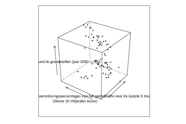
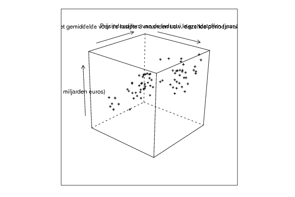
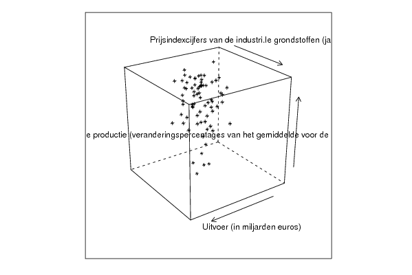
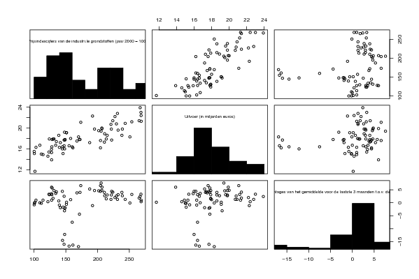
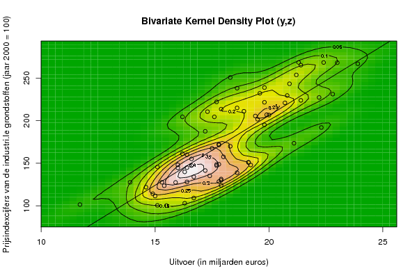
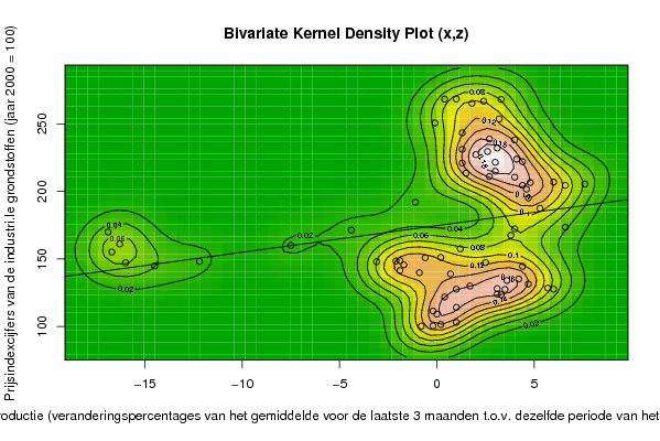
| Title produced by software | Trivariate Scatterplots | ||||||||||||||||||||
| Date of computation | Thu, 17 Dec 2009 05:05:12 -0700 | ||||||||||||||||||||
| Cite this page as follows | Statistical Computations at FreeStatistics.org, Office for Research Development and Education, URL https://freestatistics.org/blog/index.php?v=date/2009/Dec/17/t12610515798o752zyo9rc9qm5.htm/, Retrieved Tue, 30 Apr 2024 06:59:23 +0000 | ||||||||||||||||||||
| Statistical Computations at FreeStatistics.org, Office for Research Development and Education, URL https://freestatistics.org/blog/index.php?pk=68777, Retrieved Tue, 30 Apr 2024 06:59:23 +0000 | |||||||||||||||||||||
| QR Codes: | |||||||||||||||||||||
|
| |||||||||||||||||||||
| Original text written by user: | |||||||||||||||||||||
| IsPrivate? | No (this computation is public) | ||||||||||||||||||||
| User-defined keywords | SHW Paper: Trivariate scatterplots | ||||||||||||||||||||
| Estimated Impact | 165 | ||||||||||||||||||||
Tree of Dependent Computations | |||||||||||||||||||||
| Family? (F = Feedback message, R = changed R code, M = changed R Module, P = changed Parameters, D = changed Data) | |||||||||||||||||||||
| - [Trivariate Scatterplots] [WS 5 -Trivariate ...] [2009-10-28 17:50:21] [b103a1dc147def8132c7f643ad8c8f84] - MPD [Trivariate Scatterplots] [Paper: Trivariate...] [2009-12-17 12:05:12] [a45cc820faa25ce30779915639528ec2] [Current] | |||||||||||||||||||||
| Feedback Forum | |||||||||||||||||||||
Post a new message | |||||||||||||||||||||
Dataset | |||||||||||||||||||||
| Dataseries X: | |||||||||||||||||||||
-0.8 -0.2 0.2 1 0 -0.2 1 0.4 1 1.7 3.1 3.3 3.1 3.5 6 5.7 4.7 4.2 3.6 4.4 2.5 -0.6 -1.9 -1.9 0.7 -0.9 -1.7 -3.1 -2.1 0.2 1.2 3.8 4 6.6 5.3 7.6 4.7 6.6 4.4 4.6 6 4.8 4 2.7 3 4.1 4 2.7 2.6 3.1 4.4 3 2 1.3 1.5 1.3 3.2 1.8 3.3 1 2.4 0.4 -0.1 1.3 -1.1 -4.4 -7.5 -12.2 -14.5 -16 -16.7 -16.3 -16.9 | |||||||||||||||||||||
| Dataseries Y: | |||||||||||||||||||||
15,5 15,1 11,7 16,3 16,7 15 14,9 14,6 15,3 17,9 16,4 15,4 17,9 15,9 13,9 17,8 17,9 17,4 16,7 16 16,6 19,1 17,8 17,2 18,6 16,3 15,1 19,2 17,7 19,1 18 17,5 17,8 21,1 17,2 19,4 19,8 17,6 16,2 19,5 19,9 20 17,3 18,9 18,6 21,4 18,6 19,8 20,8 19,6 17,7 19,8 22,2 20,7 17,9 20,9 21,2 21,4 23 21,3 23,9 22,4 18,3 22,8 22,3 17,8 16,4 16 16,4 17,7 16,6 16,2 18,3 | |||||||||||||||||||||
| Dataseries Z: | |||||||||||||||||||||
100.2 100.4 101.4 103 109.1 111.4 114.1 121.8 127.6 129.9 128 123.5 124 127.4 127.6 128.4 131.4 135.1 134 144.5 147.3 150.9 148.7 141.4 138.9 139.8 145.6 147.9 148.5 151.1 157.5 167.5 172.3 173.5 187.5 205.5 195.1 204.5 204.5 201.7 207 206.6 210.6 211.1 215 223.9 238.2 238.9 229.6 232.2 222.1 221.6 227.3 221 213.6 243.4 253.8 265.3 268.2 268.5 266.9 268.4 250.8 231.2 192 171.4 160 148.1 144.8 147.2 155.1 161.1 169.9 | |||||||||||||||||||||
Tables (Output of Computation) | |||||||||||||||||||||
| |||||||||||||||||||||
Figures (Output of Computation) | |||||||||||||||||||||
Input Parameters & R Code | |||||||||||||||||||||
| Parameters (Session): | |||||||||||||||||||||
| par1 = 50 ; par2 = 50 ; par3 = Y ; par4 = Y ; par5 = Industri�le productie (veranderingspercentages van het gemiddelde voor de laatste 3 maanden t.o.v. dezelfde periode van het voorgaande jaar) ; par6 = Uitvoer (in miljarden euros) ; par7 = Prijsindexcijfers van de industri�le grondstoffen (jaar 2000 = 100) ; | |||||||||||||||||||||
| Parameters (R input): | |||||||||||||||||||||
| par1 = 50 ; par2 = 50 ; par3 = Y ; par4 = Y ; par5 = Industri�le productie (veranderingspercentages van het gemiddelde voor de laatste 3 maanden t.o.v. dezelfde periode van het voorgaande jaar) ; par6 = Uitvoer (in miljarden euros) ; par7 = Prijsindexcijfers van de industri�le grondstoffen (jaar 2000 = 100) ; | |||||||||||||||||||||
| R code (references can be found in the software module): | |||||||||||||||||||||
x <- array(x,dim=c(length(x),1)) | |||||||||||||||||||||