Repository of Reproducible Computations

Free Statistics

of Irreproducible Research!

Author's title

Author

*The author of this computation has been verified*

R Software Module

rwasp_multipleregression.wasp

Title produced by software

Multiple Regression

Date of computation

Sat, 21 Nov 2009 03:22:47 -0700

Cite this page as follows

Statistical Computations at FreeStatistics.org, Office for Research Development and Education, URL https://freestatistics.org/blog/index.php?v=date/2009/Nov/21/t1258799017b68tfc408ifzued.htm/, Retrieved Sun, 28 Apr 2024 06:58:42 +0000

Statistical Computations at FreeStatistics.org, Office for Research Development and Education, URL https://freestatistics.org/blog/index.php?pk=58524, Retrieved Sun, 28 Apr 2024 06:58:42 +0000

QR Codes:

Paste this QR Code to cite your computation.

Original text written by user:

IsPrivate?

No (this computation is public)

User-defined keywords

Estimated Impact

281

Family? (F = Feedback message, R = changed R code, M = changed R Module, P = changed Parameters, D = changed Data)

-     [Multiple Regression] [Q1 The Seatbeltlaw] [2007-11-14 19:27:43] [8cd6641b921d30ebe00b648d1481bba0]
- RMPD  [Multiple Regression] [Seatbelt] [2009-11-12 13:54:52] [b98453cac15ba1066b407e146608df68]
-    D    [Multiple Regression] [WS7] [2009-11-18 17:01:04] [8b1aef4e7013bd33fbc2a5833375c5f5]
-   PD      [Multiple Regression] [WS7(2)] [2009-11-20 19:01:46] [7d268329e554b8694908ba13e6e6f258]
-   P           [Multiple Regression] [WS7(3)] [2009-11-21 10:22:47] [5edea6bc5a9a9483633d9320282a2734] [Current]
-   PD            [Multiple Regression] [WS7(4)] [2009-11-21 10:55:20] [7d268329e554b8694908ba13e6e6f258] 
-    D              [Multiple Regression] [WS 7] [2009-11-25 18:27:00] [9717cb857c153ca3061376906953b329] 
- RMPD              [Univariate Data Series] [Niet-werkende wer...] [2009-11-25 19:16:52] [9717cb857c153ca3061376906953b329] 
- RMP                 [Univariate Explorative Data Analysis] [Univariate EDA] [2009-12-17 13:35:10] [9717cb857c153ca3061376906953b329] 
- RMP                   [Central Tendency] [Robustness of Cen...] [2009-12-17 22:54:55] [9717cb857c153ca3061376906953b329] 
-    D                    [Central Tendency] [Robustness of Cen...] [2009-12-29 21:57:55] [9717cb857c153ca3061376906953b329] 
-    D                  [Univariate Explorative Data Analysis] [Univariate EDA] [2009-12-29 21:52:56] [9717cb857c153ca3061376906953b329] 
-    D                  [Univariate Explorative Data Analysis] [] [2010-12-16 18:32:59] [bcc4ad4a6c0f95d5b548de29638ac6c2] 
- RMP                     [(Partial) Autocorrelation Function] [] [2010-12-16 18:42:27] [bcc4ad4a6c0f95d5b548de29638ac6c2] 
- RMP                     [(Partial) Autocorrelation Function] [] [2010-12-16 18:44:05] [bcc4ad4a6c0f95d5b548de29638ac6c2] 
- RMP                     [(Partial) Autocorrelation Function] [] [2010-12-16 18:45:46] [bcc4ad4a6c0f95d5b548de29638ac6c2] 
- RMP                     [Spectral Analysis] [] [2010-12-16 18:49:45] [bcc4ad4a6c0f95d5b548de29638ac6c2] 
- RMP                     [Spectral Analysis] [] [2010-12-16 18:50:41] [bcc4ad4a6c0f95d5b548de29638ac6c2] 
- RMP                     [Spectral Analysis] [] [2010-12-16 18:52:04] [bcc4ad4a6c0f95d5b548de29638ac6c2] 
- RMP                     [Variance Reduction Matrix] [] [2010-12-16 18:53:37] [bcc4ad4a6c0f95d5b548de29638ac6c2] 
- RMP                     [Standard Deviation-Mean Plot] [] [2010-12-16 18:55:46] [bcc4ad4a6c0f95d5b548de29638ac6c2] 
-    D                    [Univariate Explorative Data Analysis] [] [2010-12-19 14:43:39] [bcc4ad4a6c0f95d5b548de29638ac6c2] 
-   PD                  [Univariate Explorative Data Analysis] [Paper tijdreeks] [2011-12-16 15:35:08] [fbaf17a8836493f6de0f4e0e997711e1] 
-   PD                    [Univariate Explorative Data Analysis] [Paper wijn] [2011-12-17 10:19:24] [fbaf17a8836493f6de0f4e0e997711e1] 
- R PD                      [Univariate Explorative Data Analysis] [paper lag] [2011-12-18 14:28:16] [fbaf17a8836493f6de0f4e0e997711e1] 
- RMP                       [ARIMA Forecasting] [paper arima forec...] [2011-12-18 14:35:06] [fbaf17a8836493f6de0f4e0e997711e1] 
- RMPD                        [Histogram] [frequency] [2011-12-18 21:24:53] [fbaf17a8836493f6de0f4e0e997711e1] 
- RMPD                    [Central Tendency] [Paper wijn] [2011-12-17 10:31:45] [fbaf17a8836493f6de0f4e0e997711e1] 
- RMPD                    [(Partial) Autocorrelation Function] [Paper wijn] [2011-12-17 10:49:14] [fbaf17a8836493f6de0f4e0e997711e1] 
- RMPD                  [Central Tendency] [Paper tijdreeks mean] [2011-12-16 16:04:44] [fbaf17a8836493f6de0f4e0e997711e1] 
-   PD                [Univariate Data Series] [] [2010-12-16 17:58:43] [bcc4ad4a6c0f95d5b548de29638ac6c2] 
-   PD                  [Univariate Data Series] [] [2010-12-19 14:40:10] [bcc4ad4a6c0f95d5b548de29638ac6c2] 
- RMP                     [(Partial) Autocorrelation Function] [] [2010-12-19 14:45:15] [bcc4ad4a6c0f95d5b548de29638ac6c2] 
-   P                     [Univariate Data Series] [] [2010-12-19 15:24:57] [bcc4ad4a6c0f95d5b548de29638ac6c2] 
- RMP                     [(Partial) Autocorrelation Function] [] [2010-12-19 16:23:25] [bcc4ad4a6c0f95d5b548de29638ac6c2] 
- RMP                     [(Partial) Autocorrelation Function] [] [2010-12-19 16:24:34] [bcc4ad4a6c0f95d5b548de29638ac6c2] 
- RMP                     [(Partial) Autocorrelation Function] [] [2010-12-19 16:26:19] [bcc4ad4a6c0f95d5b548de29638ac6c2] 
- RMP                     [Spectral Analysis] [] [2010-12-19 16:28:33] [bcc4ad4a6c0f95d5b548de29638ac6c2] 
- RMP                     [Spectral Analysis] [] [2010-12-19 16:29:44] [bcc4ad4a6c0f95d5b548de29638ac6c2] 
- RMP                     [Spectral Analysis] [] [2010-12-19 16:30:39] [bcc4ad4a6c0f95d5b548de29638ac6c2] 
- RMP                     [Variance Reduction Matrix] [] [2010-12-19 16:33:11] [bcc4ad4a6c0f95d5b548de29638ac6c2] 
- RMP                     [Standard Deviation-Mean Plot] [] [2010-12-19 16:35:52] [bcc4ad4a6c0f95d5b548de29638ac6c2] 
- RMP                     [ARIMA Backward Selection] [] [2010-12-19 16:37:56] [bcc4ad4a6c0f95d5b548de29638ac6c2] 
- RMP                       [ARIMA Forecasting] [] [2010-12-27 23:50:02] [bcc4ad4a6c0f95d5b548de29638ac6c2] 
- RMP                     [ARIMA Forecasting] [] [2010-12-19 16:45:16] [bcc4ad4a6c0f95d5b548de29638ac6c2] 
-   PD                [Univariate Data Series] [Werloosheid bij V...] [2010-12-26 15:10:52] [e4afca2801c0b93eac84a600ed82fb9c] 
-   PD                [Univariate Data Series] [Werkloosheid vrou...] [2010-12-26 15:13:10] [e4afca2801c0b93eac84a600ed82fb9c] 

Feedback Forum

Post a new message

Dataseries X:

Download CSV

Histogram

Boxplots

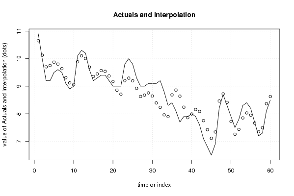
8.1	10.9
7.7	10
7.5	9.2
7.6	9.2
7.8	9.5
7.8	9.6
7.8	9.5
7.5	9.1
7.5	8.9
7.1	9
7.5	10.1
7.5	10.3
7.6	10.2
7.7	9.6
7.7	9.2
7.9	9.3
8.1	9.4
8.2	9.4
8.2	9.2
8.2	9
7.9	9
7.3	9
6.9	9.8
6.6	10
6.7	9.8
6.9	9.3
7	9
7.1	9
7.2	9.1
7.1	9.1
6.9	9.1
7	9.2
6.8	8.8
6.4	8.3
6.7	8.4
6.6	8.1
6.4	7.7
6.3	7.9
6.2	7.9
6.5	8
6.8	7.9
6.8	7.6
6.4	7.1
6.1	6.8
5.8	6.5
6.1	6.9
7.2	8.2
7.3	8.7
6.9	8.3
6.1	7.9
5.8	7.5
6.2	7.8
7.1	8.3
7.7	8.4
7.9	8.2
7.7	7.7
7.4	7.2
7.5	7.3
8	8.1
8.1	8.5

Summary of computational transaction
Raw Input	view raw input (R code)
Raw Output	view raw output of R engine
Computing time	3 seconds
R Server	'Gwilym Jenkins' @ 72.249.127.135

\begin{tabular}{lllllllll}
\hline
Summary of computational transaction \tabularnewline
Raw Input & view raw input (R code)  \tabularnewline
Raw Output & view raw output of R engine  \tabularnewline
Computing time & 3 seconds \tabularnewline
R Server & 'Gwilym Jenkins' @ 72.249.127.135 \tabularnewline
\hline
\end{tabular}
%Source: https://freestatistics.org/blog/index.php?pk=58524&T=0

[TABLE]
[ROW][C]Summary of computational transaction[/C][/ROW]
[ROW][C]Raw Input[/C][C]view raw input (R code) [/C][/ROW]
[ROW][C]Raw Output[/C][C]view raw output of R engine [/C][/ROW]
[ROW][C]Computing time[/C][C]3 seconds[/C][/ROW]
[ROW][C]R Server[/C][C]'Gwilym Jenkins' @ 72.249.127.135[/C][/ROW]
[/TABLE]
Source: https://freestatistics.org/blog/index.php?pk=58524&T=0

Globally Unique Identifier (entire table): ba.freestatistics.org/blog/index.php?pk=58524&T=0

As an alternative you can also use a QR Code:

The GUIDs for individual cells are displayed in the table below:

Summary of computational transaction
Raw Input	view raw input (R code)
Raw Output	view raw output of R engine
Computing time	3 seconds
R Server	'Gwilym Jenkins' @ 72.249.127.135

Multiple Linear Regression - Estimated Regression Equation
Werkl_Vrouwen[t] = + 7.38673263298069 + 0.4196382333358Werkl_Mannen[t] -0.10258803728638M1[t] -0.422645927350743M2[t] -0.724667640748687M3[t] -0.680973588814086M4[t] -0.607636124879781M5[t] -0.6419782496116M6[t] -0.77239272767626M7[t] -0.937628911740772M8[t] -1.08929403713842M9[t] -0.949351927202781M10[t] -0.252799992601909M11[t] -0.0360144632684767t + e[t]

\begin{tabular}{lllllllll}
\hline
Multiple Linear Regression - Estimated Regression Equation \tabularnewline
Werkl_Vrouwen[t] =  +  7.38673263298069 +  0.4196382333358Werkl_Mannen[t] -0.10258803728638M1[t] -0.422645927350743M2[t] -0.724667640748687M3[t] -0.680973588814086M4[t] -0.607636124879781M5[t] -0.6419782496116M6[t] -0.77239272767626M7[t] -0.937628911740772M8[t] -1.08929403713842M9[t] -0.949351927202781M10[t] -0.252799992601909M11[t] -0.0360144632684767t  + e[t] \tabularnewline
\hline
\end{tabular}
%Source: https://freestatistics.org/blog/index.php?pk=58524&T=1

[TABLE]
[ROW][C]Multiple Linear Regression - Estimated Regression Equation[/C][/ROW]
[ROW][C]Werkl_Vrouwen[t] =  +  7.38673263298069 +  0.4196382333358Werkl_Mannen[t] -0.10258803728638M1[t] -0.422645927350743M2[t] -0.724667640748687M3[t] -0.680973588814086M4[t] -0.607636124879781M5[t] -0.6419782496116M6[t] -0.77239272767626M7[t] -0.937628911740772M8[t] -1.08929403713842M9[t] -0.949351927202781M10[t] -0.252799992601909M11[t] -0.0360144632684767t  + e[t][/C][/ROW]
[/TABLE]
Source: https://freestatistics.org/blog/index.php?pk=58524&T=1

Globally Unique Identifier (entire table): ba.freestatistics.org/blog/index.php?pk=58524&T=1

As an alternative you can also use a QR Code:

The GUIDs for individual cells are displayed in the table below:

Multiple Linear Regression - Estimated Regression Equation
Werkl_Vrouwen[t] = + 7.38673263298069 + 0.4196382333358Werkl_Mannen[t] -0.10258803728638M1[t] -0.422645927350743M2[t] -0.724667640748687M3[t] -0.680973588814086M4[t] -0.607636124879781M5[t] -0.6419782496116M6[t] -0.77239272767626M7[t] -0.937628911740772M8[t] -1.08929403713842M9[t] -0.949351927202781M10[t] -0.252799992601909M11[t] -0.0360144632684767t + e[t]

Multiple Linear Regression - Ordinary Least Squares
Variable	Parameter	S.D.	T-STATH0: parameter = 0	2-tail p-value	1-tail p-value
(Intercept)	7.38673263298069	0.882223	8.3729	0	0
Werkl_Mannen	0.4196382333358	0.108377	3.872	0.000339	0.00017
M1	-0.10258803728638	0.294941	-0.3478	0.729557	0.364779
M2	-0.422645927350743	0.297106	-1.4225	0.161615	0.080807
M3	-0.724667640748687	0.298324	-2.4291	0.0191	0.00955
M4	-0.680973588814086	0.294082	-2.3156	0.025093	0.012546
M5	-0.607636124879781	0.292094	-2.0803	0.043098	0.021549
M6	-0.6419782496116	0.292536	-2.1945	0.033285	0.016642
M7	-0.77239272767626	0.291882	-2.6462	0.011104	0.005552
M8	-0.937628911740772	0.291328	-3.2185	0.002364	0.001182
M9	-1.08929403713842	0.291911	-3.7316	0.000522	0.000261
M10	-0.949351927202781	0.293879	-3.2304	0.002285	0.001143
M11	-0.252799992601909	0.29102	-0.8687	0.389538	0.194769
t	-0.0360144632684767	0.003953	-9.1117	0	0

\begin{tabular}{lllllllll}
\hline
Multiple Linear Regression - Ordinary Least Squares \tabularnewline
Variable & Parameter & S.D. & T-STATH0: parameter = 0 & 2-tail p-value & 1-tail p-value \tabularnewline
(Intercept) & 7.38673263298069 & 0.882223 & 8.3729 & 0 & 0 \tabularnewline
Werkl_Mannen & 0.4196382333358 & 0.108377 & 3.872 & 0.000339 & 0.00017 \tabularnewline
M1 & -0.10258803728638 & 0.294941 & -0.3478 & 0.729557 & 0.364779 \tabularnewline
M2 & -0.422645927350743 & 0.297106 & -1.4225 & 0.161615 & 0.080807 \tabularnewline
M3 & -0.724667640748687 & 0.298324 & -2.4291 & 0.0191 & 0.00955 \tabularnewline
M4 & -0.680973588814086 & 0.294082 & -2.3156 & 0.025093 & 0.012546 \tabularnewline
M5 & -0.607636124879781 & 0.292094 & -2.0803 & 0.043098 & 0.021549 \tabularnewline
M6 & -0.6419782496116 & 0.292536 & -2.1945 & 0.033285 & 0.016642 \tabularnewline
M7 & -0.77239272767626 & 0.291882 & -2.6462 & 0.011104 & 0.005552 \tabularnewline
M8 & -0.937628911740772 & 0.291328 & -3.2185 & 0.002364 & 0.001182 \tabularnewline
M9 & -1.08929403713842 & 0.291911 & -3.7316 & 0.000522 & 0.000261 \tabularnewline
M10 & -0.949351927202781 & 0.293879 & -3.2304 & 0.002285 & 0.001143 \tabularnewline
M11 & -0.252799992601909 & 0.29102 & -0.8687 & 0.389538 & 0.194769 \tabularnewline
t & -0.0360144632684767 & 0.003953 & -9.1117 & 0 & 0 \tabularnewline
\hline
\end{tabular}
%Source: https://freestatistics.org/blog/index.php?pk=58524&T=2

[TABLE]
[ROW][C]Multiple Linear Regression - Ordinary Least Squares[/C][/ROW]
[ROW][C]Variable[/C][C]Parameter[/C][C]S.D.[/C][C]T-STATH0: parameter = 0[/C][C]2-tail p-value[/C][C]1-tail p-value[/C][/ROW]
[ROW][C](Intercept)[/C][C]7.38673263298069[/C][C]0.882223[/C][C]8.3729[/C][C]0[/C][C]0[/C][/ROW]
[ROW][C]Werkl_Mannen[/C][C]0.4196382333358[/C][C]0.108377[/C][C]3.872[/C][C]0.000339[/C][C]0.00017[/C][/ROW]
[ROW][C]M1[/C][C]-0.10258803728638[/C][C]0.294941[/C][C]-0.3478[/C][C]0.729557[/C][C]0.364779[/C][/ROW]
[ROW][C]M2[/C][C]-0.422645927350743[/C][C]0.297106[/C][C]-1.4225[/C][C]0.161615[/C][C]0.080807[/C][/ROW]
[ROW][C]M3[/C][C]-0.724667640748687[/C][C]0.298324[/C][C]-2.4291[/C][C]0.0191[/C][C]0.00955[/C][/ROW]
[ROW][C]M4[/C][C]-0.680973588814086[/C][C]0.294082[/C][C]-2.3156[/C][C]0.025093[/C][C]0.012546[/C][/ROW]
[ROW][C]M5[/C][C]-0.607636124879781[/C][C]0.292094[/C][C]-2.0803[/C][C]0.043098[/C][C]0.021549[/C][/ROW]
[ROW][C]M6[/C][C]-0.6419782496116[/C][C]0.292536[/C][C]-2.1945[/C][C]0.033285[/C][C]0.016642[/C][/ROW]
[ROW][C]M7[/C][C]-0.77239272767626[/C][C]0.291882[/C][C]-2.6462[/C][C]0.011104[/C][C]0.005552[/C][/ROW]
[ROW][C]M8[/C][C]-0.937628911740772[/C][C]0.291328[/C][C]-3.2185[/C][C]0.002364[/C][C]0.001182[/C][/ROW]
[ROW][C]M9[/C][C]-1.08929403713842[/C][C]0.291911[/C][C]-3.7316[/C][C]0.000522[/C][C]0.000261[/C][/ROW]
[ROW][C]M10[/C][C]-0.949351927202781[/C][C]0.293879[/C][C]-3.2304[/C][C]0.002285[/C][C]0.001143[/C][/ROW]
[ROW][C]M11[/C][C]-0.252799992601909[/C][C]0.29102[/C][C]-0.8687[/C][C]0.389538[/C][C]0.194769[/C][/ROW]
[ROW][C]t[/C][C]-0.0360144632684767[/C][C]0.003953[/C][C]-9.1117[/C][C]0[/C][C]0[/C][/ROW]
[/TABLE]
Source: https://freestatistics.org/blog/index.php?pk=58524&T=2

Globally Unique Identifier (entire table): ba.freestatistics.org/blog/index.php?pk=58524&T=2

As an alternative you can also use a QR Code:

The GUIDs for individual cells are displayed in the table below:

Multiple Linear Regression - Ordinary Least Squares
Variable	Parameter	S.D.	T-STATH0: parameter = 0	2-tail p-value	1-tail p-value
(Intercept)	7.38673263298069	0.882223	8.3729	0	0
Werkl_Mannen	0.4196382333358	0.108377	3.872	0.000339	0.00017
M1	-0.10258803728638	0.294941	-0.3478	0.729557	0.364779
M2	-0.422645927350743	0.297106	-1.4225	0.161615	0.080807
M3	-0.724667640748687	0.298324	-2.4291	0.0191	0.00955
M4	-0.680973588814086	0.294082	-2.3156	0.025093	0.012546
M5	-0.607636124879781	0.292094	-2.0803	0.043098	0.021549
M6	-0.6419782496116	0.292536	-2.1945	0.033285	0.016642
M7	-0.77239272767626	0.291882	-2.6462	0.011104	0.005552
M8	-0.937628911740772	0.291328	-3.2185	0.002364	0.001182
M9	-1.08929403713842	0.291911	-3.7316	0.000522	0.000261
M10	-0.949351927202781	0.293879	-3.2304	0.002285	0.001143
M11	-0.252799992601909	0.29102	-0.8687	0.389538	0.194769
t	-0.0360144632684767	0.003953	-9.1117	0	0

Multiple Linear Regression - Regression Statistics
Multiple R	0.904201859845491
R-squared	0.817581003348045
Adjusted R-squared	0.766027808642058
F-TEST (value)	15.8589784398578
F-TEST (DF numerator)	13
F-TEST (DF denominator)	46
p-value	7.72271135929259e-13
Multiple Linear Regression - Residual Statistics
Residual Standard Deviation	0.460092760998810
Sum Squared Residuals	9.73752604128135

\begin{tabular}{lllllllll}
\hline
Multiple Linear Regression - Regression Statistics \tabularnewline
Multiple R & 0.904201859845491 \tabularnewline
R-squared & 0.817581003348045 \tabularnewline
Adjusted R-squared & 0.766027808642058 \tabularnewline
F-TEST (value) & 15.8589784398578 \tabularnewline
F-TEST (DF numerator) & 13 \tabularnewline
F-TEST (DF denominator) & 46 \tabularnewline
p-value & 7.72271135929259e-13 \tabularnewline
Multiple Linear Regression - Residual Statistics \tabularnewline
Residual Standard Deviation & 0.460092760998810 \tabularnewline
Sum Squared Residuals & 9.73752604128135 \tabularnewline
\hline
\end{tabular}
%Source: https://freestatistics.org/blog/index.php?pk=58524&T=3

[TABLE]
[ROW][C]Multiple Linear Regression - Regression Statistics[/C][/ROW]
[ROW][C]Multiple R[/C][C]0.904201859845491[/C][/ROW]
[ROW][C]R-squared[/C][C]0.817581003348045[/C][/ROW]
[ROW][C]Adjusted R-squared[/C][C]0.766027808642058[/C][/ROW]
[ROW][C]F-TEST (value)[/C][C]15.8589784398578[/C][/ROW]
[ROW][C]F-TEST (DF numerator)[/C][C]13[/C][/ROW]
[ROW][C]F-TEST (DF denominator)[/C][C]46[/C][/ROW]
[ROW][C]p-value[/C][C]7.72271135929259e-13[/C][/ROW]
[ROW][C]Multiple Linear Regression - Residual Statistics[/C][/ROW]
[ROW][C]Residual Standard Deviation[/C][C]0.460092760998810[/C][/ROW]
[ROW][C]Sum Squared Residuals[/C][C]9.73752604128135[/C][/ROW]
[/TABLE]
Source: https://freestatistics.org/blog/index.php?pk=58524&T=3

Globally Unique Identifier (entire table): ba.freestatistics.org/blog/index.php?pk=58524&T=3

As an alternative you can also use a QR Code:

The GUIDs for individual cells are displayed in the table below:

Multiple Linear Regression - Regression Statistics
Multiple R	0.904201859845491
R-squared	0.817581003348045
Adjusted R-squared	0.766027808642058
F-TEST (value)	15.8589784398578
F-TEST (DF numerator)	13
F-TEST (DF denominator)	46
p-value	7.72271135929259e-13
Multiple Linear Regression - Residual Statistics
Residual Standard Deviation	0.460092760998810
Sum Squared Residuals	9.73752604128135

Multiple Linear Regression - Actuals, Interpolation, and Residuals
Time or Index	Actuals	InterpolationForecast	ResidualsPrediction Error
1	10.9	10.6471998224458	0.252800177554192
2	10	10.1232721757786	-0.123272175778647
3	9.2	9.70130835244507	-0.50130835244507
4	9.2	9.75095176444477	-0.550951764444773
5	9.5	9.87220241177776	-0.372202411777762
6	9.6	9.80184582377747	-0.201845823777466
7	9.5	9.63541688244433	-0.135416882444329
8	9.1	9.3082747651106	-0.208274765110602
9	8.9	9.12059517644448	-0.220595176444477
10	9	9.05666752977732	-0.0566675297773168
11	10.1	9.88506029444403	0.214939705555966
12	10.3	10.1018458237775	0.198154176222535
13	10.2	10.0052071465562	0.19479285344381
14	9.6	9.69109861655693	-0.0910986165569288
15	9.2	9.3530624398905	-0.153062439890509
16	9.3	9.4446696752238	-0.144669675223792
17	9.4	9.56592032255678	-0.16592032255678
18	9.4	9.53752755789006	-0.137527557890064
19	9.2	9.37109861655693	-0.171098616556928
20	9	9.16984796922394	-0.169847969223940
21	9	8.85627691055708	0.143723089442923
22	9	8.70842161722276	0.291578382777243
23	9.8	9.20110379522083	0.598896204779168
24	10	9.29199785455353	0.708002145446474
25	9.8	9.19535917733225	0.604640822667752
26	9.3	8.92321447066657	0.376785529333432
27	9	8.62714211733373	0.372857882666272
28	9	8.67678552933343	0.323214470666568
29	9.1	8.75607235333284	0.343927646667159
30	9.1	8.64375194199896	0.456248058001036
31	9.1	8.39339535399867	0.706604646001332
32	9.2	8.23410852999926	0.96589147000074
33	8.8	7.96250129466598	0.837498705334024
34	8.3	7.89857364799882	0.401426352001184
35	8.4	8.68500258933195	-0.285002589331952
36	8.1	8.8598242953318	-0.759824295331805
37	7.7	8.63729414810979	-0.937294148109789
38	7.9	8.23925797144337	-0.339257971443368
39	7.9	7.85925797144337	0.0407420285566328
40	8	7.99282903011023	0.00717096988976843
41	7.9	8.1560435007768	-0.256043500776799
42	7.6	8.0856869127765	-0.485686912776504
43	7.1	7.75140267810905	-0.651402678109048
44	6.8	7.42426056077532	-0.62426056077532
45	6.5	7.11068950210846	-0.610689502108456
46	6.9	7.34050861877636	-0.440508618776356
47	8.2	8.46264814677813	-0.262648146778132
48	8.7	8.72139749944514	-0.0213974994451436
49	8.3	8.41493970555597	-0.114939705555966
50	7.9	7.72315676555449	0.176843234445513
51	7.5	7.25922911888733	0.240770881112673
52	7.8	7.43476400088777	0.365235999112229
53	8.3	7.84976141155582	0.450238588444182
54	8.4	8.031187763557	0.368812236442998
55	8.2	7.94868646889103	0.251313531108973
56	7.7	7.66350817489088	0.0364918251091230
57	7.2	7.34993711622401	-0.149937116224014
58	7.3	7.49582858622475	-0.195828586224754
59	8.1	8.36618517422505	-0.26618517422505
60	8.5	8.62493452689206	-0.124934526892061

\begin{tabular}{lllllllll}
\hline
Multiple Linear Regression - Actuals, Interpolation, and Residuals \tabularnewline
Time or Index & Actuals & InterpolationForecast & ResidualsPrediction Error \tabularnewline
1 & 10.9 & 10.6471998224458 & 0.252800177554192 \tabularnewline
2 & 10 & 10.1232721757786 & -0.123272175778647 \tabularnewline
3 & 9.2 & 9.70130835244507 & -0.50130835244507 \tabularnewline
4 & 9.2 & 9.75095176444477 & -0.550951764444773 \tabularnewline
5 & 9.5 & 9.87220241177776 & -0.372202411777762 \tabularnewline
6 & 9.6 & 9.80184582377747 & -0.201845823777466 \tabularnewline
7 & 9.5 & 9.63541688244433 & -0.135416882444329 \tabularnewline
8 & 9.1 & 9.3082747651106 & -0.208274765110602 \tabularnewline
9 & 8.9 & 9.12059517644448 & -0.220595176444477 \tabularnewline
10 & 9 & 9.05666752977732 & -0.0566675297773168 \tabularnewline
11 & 10.1 & 9.88506029444403 & 0.214939705555966 \tabularnewline
12 & 10.3 & 10.1018458237775 & 0.198154176222535 \tabularnewline
13 & 10.2 & 10.0052071465562 & 0.19479285344381 \tabularnewline
14 & 9.6 & 9.69109861655693 & -0.0910986165569288 \tabularnewline
15 & 9.2 & 9.3530624398905 & -0.153062439890509 \tabularnewline
16 & 9.3 & 9.4446696752238 & -0.144669675223792 \tabularnewline
17 & 9.4 & 9.56592032255678 & -0.16592032255678 \tabularnewline
18 & 9.4 & 9.53752755789006 & -0.137527557890064 \tabularnewline
19 & 9.2 & 9.37109861655693 & -0.171098616556928 \tabularnewline
20 & 9 & 9.16984796922394 & -0.169847969223940 \tabularnewline
21 & 9 & 8.85627691055708 & 0.143723089442923 \tabularnewline
22 & 9 & 8.70842161722276 & 0.291578382777243 \tabularnewline
23 & 9.8 & 9.20110379522083 & 0.598896204779168 \tabularnewline
24 & 10 & 9.29199785455353 & 0.708002145446474 \tabularnewline
25 & 9.8 & 9.19535917733225 & 0.604640822667752 \tabularnewline
26 & 9.3 & 8.92321447066657 & 0.376785529333432 \tabularnewline
27 & 9 & 8.62714211733373 & 0.372857882666272 \tabularnewline
28 & 9 & 8.67678552933343 & 0.323214470666568 \tabularnewline
29 & 9.1 & 8.75607235333284 & 0.343927646667159 \tabularnewline
30 & 9.1 & 8.64375194199896 & 0.456248058001036 \tabularnewline
31 & 9.1 & 8.39339535399867 & 0.706604646001332 \tabularnewline
32 & 9.2 & 8.23410852999926 & 0.96589147000074 \tabularnewline
33 & 8.8 & 7.96250129466598 & 0.837498705334024 \tabularnewline
34 & 8.3 & 7.89857364799882 & 0.401426352001184 \tabularnewline
35 & 8.4 & 8.68500258933195 & -0.285002589331952 \tabularnewline
36 & 8.1 & 8.8598242953318 & -0.759824295331805 \tabularnewline
37 & 7.7 & 8.63729414810979 & -0.937294148109789 \tabularnewline
38 & 7.9 & 8.23925797144337 & -0.339257971443368 \tabularnewline
39 & 7.9 & 7.85925797144337 & 0.0407420285566328 \tabularnewline
40 & 8 & 7.99282903011023 & 0.00717096988976843 \tabularnewline
41 & 7.9 & 8.1560435007768 & -0.256043500776799 \tabularnewline
42 & 7.6 & 8.0856869127765 & -0.485686912776504 \tabularnewline
43 & 7.1 & 7.75140267810905 & -0.651402678109048 \tabularnewline
44 & 6.8 & 7.42426056077532 & -0.62426056077532 \tabularnewline
45 & 6.5 & 7.11068950210846 & -0.610689502108456 \tabularnewline
46 & 6.9 & 7.34050861877636 & -0.440508618776356 \tabularnewline
47 & 8.2 & 8.46264814677813 & -0.262648146778132 \tabularnewline
48 & 8.7 & 8.72139749944514 & -0.0213974994451436 \tabularnewline
49 & 8.3 & 8.41493970555597 & -0.114939705555966 \tabularnewline
50 & 7.9 & 7.72315676555449 & 0.176843234445513 \tabularnewline
51 & 7.5 & 7.25922911888733 & 0.240770881112673 \tabularnewline
52 & 7.8 & 7.43476400088777 & 0.365235999112229 \tabularnewline
53 & 8.3 & 7.84976141155582 & 0.450238588444182 \tabularnewline
54 & 8.4 & 8.031187763557 & 0.368812236442998 \tabularnewline
55 & 8.2 & 7.94868646889103 & 0.251313531108973 \tabularnewline
56 & 7.7 & 7.66350817489088 & 0.0364918251091230 \tabularnewline
57 & 7.2 & 7.34993711622401 & -0.149937116224014 \tabularnewline
58 & 7.3 & 7.49582858622475 & -0.195828586224754 \tabularnewline
59 & 8.1 & 8.36618517422505 & -0.26618517422505 \tabularnewline
60 & 8.5 & 8.62493452689206 & -0.124934526892061 \tabularnewline
\hline
\end{tabular}
%Source: https://freestatistics.org/blog/index.php?pk=58524&T=4

[TABLE]
[ROW][C]Multiple Linear Regression - Actuals, Interpolation, and Residuals[/C][/ROW]
[ROW][C]Time or Index[/C][C]Actuals[/C][C]InterpolationForecast[/C][C]ResidualsPrediction Error[/C][/ROW]
[ROW][C]1[/C][C]10.9[/C][C]10.6471998224458[/C][C]0.252800177554192[/C][/ROW]
[ROW][C]2[/C][C]10[/C][C]10.1232721757786[/C][C]-0.123272175778647[/C][/ROW]
[ROW][C]3[/C][C]9.2[/C][C]9.70130835244507[/C][C]-0.50130835244507[/C][/ROW]
[ROW][C]4[/C][C]9.2[/C][C]9.75095176444477[/C][C]-0.550951764444773[/C][/ROW]
[ROW][C]5[/C][C]9.5[/C][C]9.87220241177776[/C][C]-0.372202411777762[/C][/ROW]
[ROW][C]6[/C][C]9.6[/C][C]9.80184582377747[/C][C]-0.201845823777466[/C][/ROW]
[ROW][C]7[/C][C]9.5[/C][C]9.63541688244433[/C][C]-0.135416882444329[/C][/ROW]
[ROW][C]8[/C][C]9.1[/C][C]9.3082747651106[/C][C]-0.208274765110602[/C][/ROW]
[ROW][C]9[/C][C]8.9[/C][C]9.12059517644448[/C][C]-0.220595176444477[/C][/ROW]
[ROW][C]10[/C][C]9[/C][C]9.05666752977732[/C][C]-0.0566675297773168[/C][/ROW]
[ROW][C]11[/C][C]10.1[/C][C]9.88506029444403[/C][C]0.214939705555966[/C][/ROW]
[ROW][C]12[/C][C]10.3[/C][C]10.1018458237775[/C][C]0.198154176222535[/C][/ROW]
[ROW][C]13[/C][C]10.2[/C][C]10.0052071465562[/C][C]0.19479285344381[/C][/ROW]
[ROW][C]14[/C][C]9.6[/C][C]9.69109861655693[/C][C]-0.0910986165569288[/C][/ROW]
[ROW][C]15[/C][C]9.2[/C][C]9.3530624398905[/C][C]-0.153062439890509[/C][/ROW]
[ROW][C]16[/C][C]9.3[/C][C]9.4446696752238[/C][C]-0.144669675223792[/C][/ROW]
[ROW][C]17[/C][C]9.4[/C][C]9.56592032255678[/C][C]-0.16592032255678[/C][/ROW]
[ROW][C]18[/C][C]9.4[/C][C]9.53752755789006[/C][C]-0.137527557890064[/C][/ROW]
[ROW][C]19[/C][C]9.2[/C][C]9.37109861655693[/C][C]-0.171098616556928[/C][/ROW]
[ROW][C]20[/C][C]9[/C][C]9.16984796922394[/C][C]-0.169847969223940[/C][/ROW]
[ROW][C]21[/C][C]9[/C][C]8.85627691055708[/C][C]0.143723089442923[/C][/ROW]
[ROW][C]22[/C][C]9[/C][C]8.70842161722276[/C][C]0.291578382777243[/C][/ROW]
[ROW][C]23[/C][C]9.8[/C][C]9.20110379522083[/C][C]0.598896204779168[/C][/ROW]
[ROW][C]24[/C][C]10[/C][C]9.29199785455353[/C][C]0.708002145446474[/C][/ROW]
[ROW][C]25[/C][C]9.8[/C][C]9.19535917733225[/C][C]0.604640822667752[/C][/ROW]
[ROW][C]26[/C][C]9.3[/C][C]8.92321447066657[/C][C]0.376785529333432[/C][/ROW]
[ROW][C]27[/C][C]9[/C][C]8.62714211733373[/C][C]0.372857882666272[/C][/ROW]
[ROW][C]28[/C][C]9[/C][C]8.67678552933343[/C][C]0.323214470666568[/C][/ROW]
[ROW][C]29[/C][C]9.1[/C][C]8.75607235333284[/C][C]0.343927646667159[/C][/ROW]
[ROW][C]30[/C][C]9.1[/C][C]8.64375194199896[/C][C]0.456248058001036[/C][/ROW]
[ROW][C]31[/C][C]9.1[/C][C]8.39339535399867[/C][C]0.706604646001332[/C][/ROW]
[ROW][C]32[/C][C]9.2[/C][C]8.23410852999926[/C][C]0.96589147000074[/C][/ROW]
[ROW][C]33[/C][C]8.8[/C][C]7.96250129466598[/C][C]0.837498705334024[/C][/ROW]
[ROW][C]34[/C][C]8.3[/C][C]7.89857364799882[/C][C]0.401426352001184[/C][/ROW]
[ROW][C]35[/C][C]8.4[/C][C]8.68500258933195[/C][C]-0.285002589331952[/C][/ROW]
[ROW][C]36[/C][C]8.1[/C][C]8.8598242953318[/C][C]-0.759824295331805[/C][/ROW]
[ROW][C]37[/C][C]7.7[/C][C]8.63729414810979[/C][C]-0.937294148109789[/C][/ROW]
[ROW][C]38[/C][C]7.9[/C][C]8.23925797144337[/C][C]-0.339257971443368[/C][/ROW]
[ROW][C]39[/C][C]7.9[/C][C]7.85925797144337[/C][C]0.0407420285566328[/C][/ROW]
[ROW][C]40[/C][C]8[/C][C]7.99282903011023[/C][C]0.00717096988976843[/C][/ROW]
[ROW][C]41[/C][C]7.9[/C][C]8.1560435007768[/C][C]-0.256043500776799[/C][/ROW]
[ROW][C]42[/C][C]7.6[/C][C]8.0856869127765[/C][C]-0.485686912776504[/C][/ROW]
[ROW][C]43[/C][C]7.1[/C][C]7.75140267810905[/C][C]-0.651402678109048[/C][/ROW]
[ROW][C]44[/C][C]6.8[/C][C]7.42426056077532[/C][C]-0.62426056077532[/C][/ROW]
[ROW][C]45[/C][C]6.5[/C][C]7.11068950210846[/C][C]-0.610689502108456[/C][/ROW]
[ROW][C]46[/C][C]6.9[/C][C]7.34050861877636[/C][C]-0.440508618776356[/C][/ROW]
[ROW][C]47[/C][C]8.2[/C][C]8.46264814677813[/C][C]-0.262648146778132[/C][/ROW]
[ROW][C]48[/C][C]8.7[/C][C]8.72139749944514[/C][C]-0.0213974994451436[/C][/ROW]
[ROW][C]49[/C][C]8.3[/C][C]8.41493970555597[/C][C]-0.114939705555966[/C][/ROW]
[ROW][C]50[/C][C]7.9[/C][C]7.72315676555449[/C][C]0.176843234445513[/C][/ROW]
[ROW][C]51[/C][C]7.5[/C][C]7.25922911888733[/C][C]0.240770881112673[/C][/ROW]
[ROW][C]52[/C][C]7.8[/C][C]7.43476400088777[/C][C]0.365235999112229[/C][/ROW]
[ROW][C]53[/C][C]8.3[/C][C]7.84976141155582[/C][C]0.450238588444182[/C][/ROW]
[ROW][C]54[/C][C]8.4[/C][C]8.031187763557[/C][C]0.368812236442998[/C][/ROW]
[ROW][C]55[/C][C]8.2[/C][C]7.94868646889103[/C][C]0.251313531108973[/C][/ROW]
[ROW][C]56[/C][C]7.7[/C][C]7.66350817489088[/C][C]0.0364918251091230[/C][/ROW]
[ROW][C]57[/C][C]7.2[/C][C]7.34993711622401[/C][C]-0.149937116224014[/C][/ROW]
[ROW][C]58[/C][C]7.3[/C][C]7.49582858622475[/C][C]-0.195828586224754[/C][/ROW]
[ROW][C]59[/C][C]8.1[/C][C]8.36618517422505[/C][C]-0.26618517422505[/C][/ROW]
[ROW][C]60[/C][C]8.5[/C][C]8.62493452689206[/C][C]-0.124934526892061[/C][/ROW]
[/TABLE]
Source: https://freestatistics.org/blog/index.php?pk=58524&T=4

Globally Unique Identifier (entire table): ba.freestatistics.org/blog/index.php?pk=58524&T=4

As an alternative you can also use a QR Code:

The GUIDs for individual cells are displayed in the table below:

Multiple Linear Regression - Actuals, Interpolation, and Residuals
Time or Index	Actuals	InterpolationForecast	ResidualsPrediction Error
1	10.9	10.6471998224458	0.252800177554192
2	10	10.1232721757786	-0.123272175778647
3	9.2	9.70130835244507	-0.50130835244507
4	9.2	9.75095176444477	-0.550951764444773
5	9.5	9.87220241177776	-0.372202411777762
6	9.6	9.80184582377747	-0.201845823777466
7	9.5	9.63541688244433	-0.135416882444329
8	9.1	9.3082747651106	-0.208274765110602
9	8.9	9.12059517644448	-0.220595176444477
10	9	9.05666752977732	-0.0566675297773168
11	10.1	9.88506029444403	0.214939705555966
12	10.3	10.1018458237775	0.198154176222535
13	10.2	10.0052071465562	0.19479285344381
14	9.6	9.69109861655693	-0.0910986165569288
15	9.2	9.3530624398905	-0.153062439890509
16	9.3	9.4446696752238	-0.144669675223792
17	9.4	9.56592032255678	-0.16592032255678
18	9.4	9.53752755789006	-0.137527557890064
19	9.2	9.37109861655693	-0.171098616556928
20	9	9.16984796922394	-0.169847969223940
21	9	8.85627691055708	0.143723089442923
22	9	8.70842161722276	0.291578382777243
23	9.8	9.20110379522083	0.598896204779168
24	10	9.29199785455353	0.708002145446474
25	9.8	9.19535917733225	0.604640822667752
26	9.3	8.92321447066657	0.376785529333432
27	9	8.62714211733373	0.372857882666272
28	9	8.67678552933343	0.323214470666568
29	9.1	8.75607235333284	0.343927646667159
30	9.1	8.64375194199896	0.456248058001036
31	9.1	8.39339535399867	0.706604646001332
32	9.2	8.23410852999926	0.96589147000074
33	8.8	7.96250129466598	0.837498705334024
34	8.3	7.89857364799882	0.401426352001184
35	8.4	8.68500258933195	-0.285002589331952
36	8.1	8.8598242953318	-0.759824295331805
37	7.7	8.63729414810979	-0.937294148109789
38	7.9	8.23925797144337	-0.339257971443368
39	7.9	7.85925797144337	0.0407420285566328
40	8	7.99282903011023	0.00717096988976843
41	7.9	8.1560435007768	-0.256043500776799
42	7.6	8.0856869127765	-0.485686912776504
43	7.1	7.75140267810905	-0.651402678109048
44	6.8	7.42426056077532	-0.62426056077532
45	6.5	7.11068950210846	-0.610689502108456
46	6.9	7.34050861877636	-0.440508618776356
47	8.2	8.46264814677813	-0.262648146778132
48	8.7	8.72139749944514	-0.0213974994451436
49	8.3	8.41493970555597	-0.114939705555966
50	7.9	7.72315676555449	0.176843234445513
51	7.5	7.25922911888733	0.240770881112673
52	7.8	7.43476400088777	0.365235999112229
53	8.3	7.84976141155582	0.450238588444182
54	8.4	8.031187763557	0.368812236442998
55	8.2	7.94868646889103	0.251313531108973
56	7.7	7.66350817489088	0.0364918251091230
57	7.2	7.34993711622401	-0.149937116224014
58	7.3	7.49582858622475	-0.195828586224754
59	8.1	8.36618517422505	-0.26618517422505
60	8.5	8.62493452689206	-0.124934526892061

Goldfeld-Quandt test for Heteroskedasticity
p-values	Alternative Hypothesis
breakpoint index	greater	2-sided	less
17	0.00730236631593619	0.0146047326318724	0.992697633684064
18	0.00558196564698079	0.0111639312939616	0.99441803435302
19	0.00421079582555247	0.00842159165110495	0.995789204174448
20	0.00216226129454762	0.00432452258909523	0.997837738705452
21	0.00123579162805974	0.00247158325611948	0.99876420837194
22	0.0005752570758167	0.0011505141516334	0.999424742924183
23	0.000363186087516210	0.000726372175032419	0.999636813912484
24	0.000292905158009509	0.000585810316019017	0.99970709484199
25	0.000154651226420498	0.000309302452840996	0.99984534877358
26	4.75697262196118e-05	9.51394524392236e-05	0.99995243027378
27	5.93322587777853e-05	0.000118664517555571	0.999940667741222
28	4.95175949780294e-05	9.90351899560588e-05	0.999950482405022
29	1.99749660869559e-05	3.99499321739117e-05	0.999980025033913
30	6.26152881613905e-06	1.25230576322781e-05	0.999993738471184
31	7.78773661908973e-06	1.55754732381795e-05	0.99999221226338
32	0.000252129175434248	0.000504258350868497	0.999747870824566
33	0.00185876586830969	0.00371753173661938	0.99814123413169
34	0.0557231348710124	0.111446269742025	0.944276865128988
35	0.70949905529625	0.5810018894075	0.29050094470375
36	0.934143729408794	0.131712541182412	0.0658562705912062
37	0.985089486888441	0.0298210262231174	0.0149105131115587
38	0.975983400952765	0.0480331980944704	0.0240165990472352
39	0.949433076178772	0.101133847642456	0.0505669238212278
40	0.899978058192927	0.200043883614146	0.100021941807073
41	0.902825530240147	0.194348939519706	0.0971744697598529
42	0.977295320584494	0.0454093588310114	0.0227046794155057
43	0.992680902802453	0.014638194395095	0.0073190971975475

\begin{tabular}{lllllllll}
\hline
Goldfeld-Quandt test for Heteroskedasticity \tabularnewline
p-values & Alternative Hypothesis \tabularnewline
breakpoint index & greater & 2-sided & less \tabularnewline
17 & 0.00730236631593619 & 0.0146047326318724 & 0.992697633684064 \tabularnewline
18 & 0.00558196564698079 & 0.0111639312939616 & 0.99441803435302 \tabularnewline
19 & 0.00421079582555247 & 0.00842159165110495 & 0.995789204174448 \tabularnewline
20 & 0.00216226129454762 & 0.00432452258909523 & 0.997837738705452 \tabularnewline
21 & 0.00123579162805974 & 0.00247158325611948 & 0.99876420837194 \tabularnewline
22 & 0.0005752570758167 & 0.0011505141516334 & 0.999424742924183 \tabularnewline
23 & 0.000363186087516210 & 0.000726372175032419 & 0.999636813912484 \tabularnewline
24 & 0.000292905158009509 & 0.000585810316019017 & 0.99970709484199 \tabularnewline
25 & 0.000154651226420498 & 0.000309302452840996 & 0.99984534877358 \tabularnewline
26 & 4.75697262196118e-05 & 9.51394524392236e-05 & 0.99995243027378 \tabularnewline
27 & 5.93322587777853e-05 & 0.000118664517555571 & 0.999940667741222 \tabularnewline
28 & 4.95175949780294e-05 & 9.90351899560588e-05 & 0.999950482405022 \tabularnewline
29 & 1.99749660869559e-05 & 3.99499321739117e-05 & 0.999980025033913 \tabularnewline
30 & 6.26152881613905e-06 & 1.25230576322781e-05 & 0.999993738471184 \tabularnewline
31 & 7.78773661908973e-06 & 1.55754732381795e-05 & 0.99999221226338 \tabularnewline
32 & 0.000252129175434248 & 0.000504258350868497 & 0.999747870824566 \tabularnewline
33 & 0.00185876586830969 & 0.00371753173661938 & 0.99814123413169 \tabularnewline
34 & 0.0557231348710124 & 0.111446269742025 & 0.944276865128988 \tabularnewline
35 & 0.70949905529625 & 0.5810018894075 & 0.29050094470375 \tabularnewline
36 & 0.934143729408794 & 0.131712541182412 & 0.0658562705912062 \tabularnewline
37 & 0.985089486888441 & 0.0298210262231174 & 0.0149105131115587 \tabularnewline
38 & 0.975983400952765 & 0.0480331980944704 & 0.0240165990472352 \tabularnewline
39 & 0.949433076178772 & 0.101133847642456 & 0.0505669238212278 \tabularnewline
40 & 0.899978058192927 & 0.200043883614146 & 0.100021941807073 \tabularnewline
41 & 0.902825530240147 & 0.194348939519706 & 0.0971744697598529 \tabularnewline
42 & 0.977295320584494 & 0.0454093588310114 & 0.0227046794155057 \tabularnewline
43 & 0.992680902802453 & 0.014638194395095 & 0.0073190971975475 \tabularnewline
\hline
\end{tabular}
%Source: https://freestatistics.org/blog/index.php?pk=58524&T=5

[TABLE]
[ROW][C]Goldfeld-Quandt test for Heteroskedasticity[/C][/ROW]
[ROW][C]p-values[/C][C]Alternative Hypothesis[/C][/ROW]
[ROW][C]breakpoint index[/C][C]greater[/C][C]2-sided[/C][C]less[/C][/ROW]
[ROW][C]17[/C][C]0.00730236631593619[/C][C]0.0146047326318724[/C][C]0.992697633684064[/C][/ROW]
[ROW][C]18[/C][C]0.00558196564698079[/C][C]0.0111639312939616[/C][C]0.99441803435302[/C][/ROW]
[ROW][C]19[/C][C]0.00421079582555247[/C][C]0.00842159165110495[/C][C]0.995789204174448[/C][/ROW]
[ROW][C]20[/C][C]0.00216226129454762[/C][C]0.00432452258909523[/C][C]0.997837738705452[/C][/ROW]
[ROW][C]21[/C][C]0.00123579162805974[/C][C]0.00247158325611948[/C][C]0.99876420837194[/C][/ROW]
[ROW][C]22[/C][C]0.0005752570758167[/C][C]0.0011505141516334[/C][C]0.999424742924183[/C][/ROW]
[ROW][C]23[/C][C]0.000363186087516210[/C][C]0.000726372175032419[/C][C]0.999636813912484[/C][/ROW]
[ROW][C]24[/C][C]0.000292905158009509[/C][C]0.000585810316019017[/C][C]0.99970709484199[/C][/ROW]
[ROW][C]25[/C][C]0.000154651226420498[/C][C]0.000309302452840996[/C][C]0.99984534877358[/C][/ROW]
[ROW][C]26[/C][C]4.75697262196118e-05[/C][C]9.51394524392236e-05[/C][C]0.99995243027378[/C][/ROW]
[ROW][C]27[/C][C]5.93322587777853e-05[/C][C]0.000118664517555571[/C][C]0.999940667741222[/C][/ROW]
[ROW][C]28[/C][C]4.95175949780294e-05[/C][C]9.90351899560588e-05[/C][C]0.999950482405022[/C][/ROW]
[ROW][C]29[/C][C]1.99749660869559e-05[/C][C]3.99499321739117e-05[/C][C]0.999980025033913[/C][/ROW]
[ROW][C]30[/C][C]6.26152881613905e-06[/C][C]1.25230576322781e-05[/C][C]0.999993738471184[/C][/ROW]
[ROW][C]31[/C][C]7.78773661908973e-06[/C][C]1.55754732381795e-05[/C][C]0.99999221226338[/C][/ROW]
[ROW][C]32[/C][C]0.000252129175434248[/C][C]0.000504258350868497[/C][C]0.999747870824566[/C][/ROW]
[ROW][C]33[/C][C]0.00185876586830969[/C][C]0.00371753173661938[/C][C]0.99814123413169[/C][/ROW]
[ROW][C]34[/C][C]0.0557231348710124[/C][C]0.111446269742025[/C][C]0.944276865128988[/C][/ROW]
[ROW][C]35[/C][C]0.70949905529625[/C][C]0.5810018894075[/C][C]0.29050094470375[/C][/ROW]
[ROW][C]36[/C][C]0.934143729408794[/C][C]0.131712541182412[/C][C]0.0658562705912062[/C][/ROW]
[ROW][C]37[/C][C]0.985089486888441[/C][C]0.0298210262231174[/C][C]0.0149105131115587[/C][/ROW]
[ROW][C]38[/C][C]0.975983400952765[/C][C]0.0480331980944704[/C][C]0.0240165990472352[/C][/ROW]
[ROW][C]39[/C][C]0.949433076178772[/C][C]0.101133847642456[/C][C]0.0505669238212278[/C][/ROW]
[ROW][C]40[/C][C]0.899978058192927[/C][C]0.200043883614146[/C][C]0.100021941807073[/C][/ROW]
[ROW][C]41[/C][C]0.902825530240147[/C][C]0.194348939519706[/C][C]0.0971744697598529[/C][/ROW]
[ROW][C]42[/C][C]0.977295320584494[/C][C]0.0454093588310114[/C][C]0.0227046794155057[/C][/ROW]
[ROW][C]43[/C][C]0.992680902802453[/C][C]0.014638194395095[/C][C]0.0073190971975475[/C][/ROW]
[/TABLE]
Source: https://freestatistics.org/blog/index.php?pk=58524&T=5

Globally Unique Identifier (entire table): ba.freestatistics.org/blog/index.php?pk=58524&T=5

As an alternative you can also use a QR Code:

The GUIDs for individual cells are displayed in the table below:

Goldfeld-Quandt test for Heteroskedasticity
p-values	Alternative Hypothesis
breakpoint index	greater	2-sided	less
17	0.00730236631593619	0.0146047326318724	0.992697633684064
18	0.00558196564698079	0.0111639312939616	0.99441803435302
19	0.00421079582555247	0.00842159165110495	0.995789204174448
20	0.00216226129454762	0.00432452258909523	0.997837738705452
21	0.00123579162805974	0.00247158325611948	0.99876420837194
22	0.0005752570758167	0.0011505141516334	0.999424742924183
23	0.000363186087516210	0.000726372175032419	0.999636813912484
24	0.000292905158009509	0.000585810316019017	0.99970709484199
25	0.000154651226420498	0.000309302452840996	0.99984534877358
26	4.75697262196118e-05	9.51394524392236e-05	0.99995243027378
27	5.93322587777853e-05	0.000118664517555571	0.999940667741222
28	4.95175949780294e-05	9.90351899560588e-05	0.999950482405022
29	1.99749660869559e-05	3.99499321739117e-05	0.999980025033913
30	6.26152881613905e-06	1.25230576322781e-05	0.999993738471184
31	7.78773661908973e-06	1.55754732381795e-05	0.99999221226338
32	0.000252129175434248	0.000504258350868497	0.999747870824566
33	0.00185876586830969	0.00371753173661938	0.99814123413169
34	0.0557231348710124	0.111446269742025	0.944276865128988
35	0.70949905529625	0.5810018894075	0.29050094470375
36	0.934143729408794	0.131712541182412	0.0658562705912062
37	0.985089486888441	0.0298210262231174	0.0149105131115587
38	0.975983400952765	0.0480331980944704	0.0240165990472352
39	0.949433076178772	0.101133847642456	0.0505669238212278
40	0.899978058192927	0.200043883614146	0.100021941807073
41	0.902825530240147	0.194348939519706	0.0971744697598529
42	0.977295320584494	0.0454093588310114	0.0227046794155057
43	0.992680902802453	0.014638194395095	0.0073190971975475

Meta Analysis of Goldfeld-Quandt test for Heteroskedasticity
Description	# significant tests	% significant tests	OK/NOK
1% type I error level	15	0.555555555555556	NOK
5% type I error level	21	0.777777777777778	NOK
10% type I error level	21	0.777777777777778	NOK

\begin{tabular}{lllllllll}
\hline
Meta Analysis of Goldfeld-Quandt test for Heteroskedasticity \tabularnewline
Description & # significant tests & % significant tests & OK/NOK \tabularnewline
1% type I error level & 15 & 0.555555555555556 & NOK \tabularnewline
5% type I error level & 21 & 0.777777777777778 & NOK \tabularnewline
10% type I error level & 21 & 0.777777777777778 & NOK \tabularnewline
\hline
\end{tabular}
%Source: https://freestatistics.org/blog/index.php?pk=58524&T=6

[TABLE]
[ROW][C]Meta Analysis of Goldfeld-Quandt test for Heteroskedasticity[/C][/ROW]
[ROW][C]Description[/C][C]# significant tests[/C][C]% significant tests[/C][C]OK/NOK[/C][/ROW]
[ROW][C]1% type I error level[/C][C]15[/C][C]0.555555555555556[/C][C]NOK[/C][/ROW]
[ROW][C]5% type I error level[/C][C]21[/C][C]0.777777777777778[/C][C]NOK[/C][/ROW]
[ROW][C]10% type I error level[/C][C]21[/C][C]0.777777777777778[/C][C]NOK[/C][/ROW]
[/TABLE]
Source: https://freestatistics.org/blog/index.php?pk=58524&T=6

Globally Unique Identifier (entire table): ba.freestatistics.org/blog/index.php?pk=58524&T=6

As an alternative you can also use a QR Code:

The GUIDs for individual cells are displayed in the table below:

Meta Analysis of Goldfeld-Quandt test for Heteroskedasticity
Description	# significant tests	% significant tests	OK/NOK
1% type I error level	15	0.555555555555556	NOK
5% type I error level	21	0.777777777777778	NOK
10% type I error level	21	0.777777777777778	NOK

Figure 1

PNG link

Postscript link

PDF link

Figure 2

PNG link

Postscript link

PDF link

Figure 3

PNG link

Postscript link

PDF link

Figure 4

PNG link

Postscript link

PDF link

Figure 5

PNG link

Postscript link

PDF link

Figure 6

PNG link

Postscript link

PDF link

Figure 7

PNG link

Postscript link

PDF link

Figure 8

PNG link

Postscript link

PDF link

Figure 9

PNG link

Postscript link

PDF link

Figure 10

PNG link

Postscript link

PDF link

Parameters (Session):

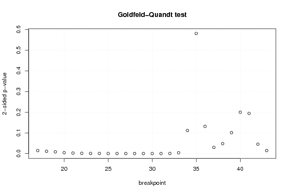
par1 = 2 ; par2 = Include Monthly Dummies ; par3 = Linear Trend ;

Parameters (R input):

par1 = 2 ; par2 = Include Monthly Dummies ; par3 = Linear Trend ;

R code (references can be found in the software module):

library(lattice)
library(lmtest)
n25 <- 25 #minimum number of obs. for Goldfeld-Quandt test
par1 <- as.numeric(par1)
x <- t(y)
k <- length(x[1,])
n <- length(x[,1])
x1 <- cbind(x[,par1], x[,1:k!=par1])
mycolnames <- c(colnames(x)[par1], colnames(x)[1:k!=par1])
colnames(x1) <- mycolnames #colnames(x)[par1]
x <- x1
if (par3 == 'First Differences'){
x2 <- array(0, dim=c(n-1,k), dimnames=list(1:(n-1), paste('(1-B)',colnames(x),sep='')))
for (i in 1:n-1) {
for (j in 1:k) {
x2[i,j] <- x[i+1,j] - x[i,j]
}
}
x <- x2
}
if (par2 == 'Include Monthly Dummies'){
x2 <- array(0, dim=c(n,11), dimnames=list(1:n, paste('M', seq(1:11), sep ='')))
for (i in 1:11){
x2[seq(i,n,12),i] <- 1
}
x <- cbind(x, x2)
}
if (par2 == 'Include Quarterly Dummies'){
x2 <- array(0, dim=c(n,3), dimnames=list(1:n, paste('Q', seq(1:3), sep ='')))
for (i in 1:3){
x2[seq(i,n,4),i] <- 1
}
x <- cbind(x, x2)
}
k <- length(x[1,])
if (par3 == 'Linear Trend'){
x <- cbind(x, c(1:n))
colnames(x)[k+1] <- 't'
}
x
k <- length(x[1,])
df <- as.data.frame(x)
(mylm <- lm(df))
(mysum <- summary(mylm))
if (n > n25) {
kp3 <- k + 3
nmkm3 <- n - k - 3
gqarr <- array(NA, dim=c(nmkm3-kp3+1,3))
numgqtests <- 0
numsignificant1 <- 0
numsignificant5 <- 0
numsignificant10 <- 0
for (mypoint in kp3:nmkm3) {
j <- 0
numgqtests <- numgqtests + 1
for (myalt in c('greater', 'two.sided', 'less')) {
j <- j + 1
gqarr[mypoint-kp3+1,j] <- gqtest(mylm, point=mypoint, alternative=myalt)$p.value
}
if (gqarr[mypoint-kp3+1,2] < 0.01) numsignificant1 <- numsignificant1 + 1
if (gqarr[mypoint-kp3+1,2] < 0.05) numsignificant5 <- numsignificant5 + 1
if (gqarr[mypoint-kp3+1,2] < 0.10) numsignificant10 <- numsignificant10 + 1
}
gqarr
}
bitmap(file='test0.png')
plot(x[,1], type='l', main='Actuals and Interpolation', ylab='value of Actuals and Interpolation (dots)', xlab='time or index')
points(x[,1]-mysum$resid)
grid()
dev.off()
bitmap(file='test1.png')
plot(mysum$resid, type='b', pch=19, main='Residuals', ylab='value of Residuals', xlab='time or index')
grid()
dev.off()
bitmap(file='test2.png')
hist(mysum$resid, main='Residual Histogram', xlab='values of Residuals')
grid()
dev.off()
bitmap(file='test3.png')
densityplot(~mysum$resid,col='black',main='Residual Density Plot', xlab='values of Residuals')
dev.off()
bitmap(file='test4.png')
qqnorm(mysum$resid, main='Residual Normal Q-Q Plot')
qqline(mysum$resid)
grid()
dev.off()
(myerror <- as.ts(mysum$resid))
bitmap(file='test5.png')
dum <- cbind(lag(myerror,k=1),myerror)
dum
dum1 <- dum[2:length(myerror),]
dum1
z <- as.data.frame(dum1)
z
plot(z,main=paste('Residual Lag plot, lowess, and regression line'), ylab='values of Residuals', xlab='lagged values of Residuals')
lines(lowess(z))
abline(lm(z))
grid()
dev.off()
bitmap(file='test6.png')
acf(mysum$resid, lag.max=length(mysum$resid)/2, main='Residual Autocorrelation Function')
grid()
dev.off()
bitmap(file='test7.png')
pacf(mysum$resid, lag.max=length(mysum$resid)/2, main='Residual Partial Autocorrelation Function')
grid()
dev.off()
bitmap(file='test8.png')
opar <- par(mfrow = c(2,2), oma = c(0, 0, 1.1, 0))
plot(mylm, las = 1, sub='Residual Diagnostics')
par(opar)
dev.off()
if (n > n25) {
bitmap(file='test9.png')
plot(kp3:nmkm3,gqarr[,2], main='Goldfeld-Quandt test',ylab='2-sided p-value',xlab='breakpoint')
grid()
dev.off()
}
load(file='createtable')
a<-table.start()
a<-table.row.start(a)
a<-table.element(a, 'Multiple Linear Regression - Estimated Regression Equation', 1, TRUE)
a<-table.row.end(a)
myeq <- colnames(x)[1]
myeq <- paste(myeq, '[t] = ', sep='')
for (i in 1:k){
if (mysum$coefficients[i,1] > 0) myeq <- paste(myeq, '+', '')
myeq <- paste(myeq, mysum$coefficients[i,1], sep=' ')
if (rownames(mysum$coefficients)[i] != '(Intercept)') {
myeq <- paste(myeq, rownames(mysum$coefficients)[i], sep='')
if (rownames(mysum$coefficients)[i] != 't') myeq <- paste(myeq, '[t]', sep='')
}
}
myeq <- paste(myeq, ' + e[t]')
a<-table.row.start(a)
a<-table.element(a, myeq)
a<-table.row.end(a)
a<-table.end(a)
table.save(a,file='mytable1.tab')
a<-table.start()
a<-table.row.start(a)
a<-table.element(a,hyperlink('ols1.htm','Multiple Linear Regression - Ordinary Least Squares',''), 6, TRUE)
a<-table.row.end(a)
a<-table.row.start(a)
a<-table.element(a,'Variable',header=TRUE)
a<-table.element(a,'Parameter',header=TRUE)
a<-table.element(a,'S.D.',header=TRUE)
a<-table.element(a,'T-STAT
H0: parameter = 0',header=TRUE)
a<-table.element(a,'2-tail p-value',header=TRUE)
a<-table.element(a,'1-tail p-value',header=TRUE)
a<-table.row.end(a)
for (i in 1:k){
a<-table.row.start(a)
a<-table.element(a,rownames(mysum$coefficients)[i],header=TRUE)
a<-table.element(a,mysum$coefficients[i,1])
a<-table.element(a, round(mysum$coefficients[i,2],6))
a<-table.element(a, round(mysum$coefficients[i,3],4))
a<-table.element(a, round(mysum$coefficients[i,4],6))
a<-table.element(a, round(mysum$coefficients[i,4]/2,6))
a<-table.row.end(a)
}
a<-table.end(a)
table.save(a,file='mytable2.tab')
a<-table.start()
a<-table.row.start(a)
a<-table.element(a, 'Multiple Linear Regression - Regression Statistics', 2, TRUE)
a<-table.row.end(a)
a<-table.row.start(a)
a<-table.element(a, 'Multiple R',1,TRUE)
a<-table.element(a, sqrt(mysum$r.squared))
a<-table.row.end(a)
a<-table.row.start(a)
a<-table.element(a, 'R-squared',1,TRUE)
a<-table.element(a, mysum$r.squared)
a<-table.row.end(a)
a<-table.row.start(a)
a<-table.element(a, 'Adjusted R-squared',1,TRUE)
a<-table.element(a, mysum$adj.r.squared)
a<-table.row.end(a)
a<-table.row.start(a)
a<-table.element(a, 'F-TEST (value)',1,TRUE)
a<-table.element(a, mysum$fstatistic[1])
a<-table.row.end(a)
a<-table.row.start(a)
a<-table.element(a, 'F-TEST (DF numerator)',1,TRUE)
a<-table.element(a, mysum$fstatistic[2])
a<-table.row.end(a)
a<-table.row.start(a)
a<-table.element(a, 'F-TEST (DF denominator)',1,TRUE)
a<-table.element(a, mysum$fstatistic[3])
a<-table.row.end(a)
a<-table.row.start(a)
a<-table.element(a, 'p-value',1,TRUE)
a<-table.element(a, 1-pf(mysum$fstatistic[1],mysum$fstatistic[2],mysum$fstatistic[3]))
a<-table.row.end(a)
a<-table.row.start(a)
a<-table.element(a, 'Multiple Linear Regression - Residual Statistics', 2, TRUE)
a<-table.row.end(a)
a<-table.row.start(a)
a<-table.element(a, 'Residual Standard Deviation',1,TRUE)
a<-table.element(a, mysum$sigma)
a<-table.row.end(a)
a<-table.row.start(a)
a<-table.element(a, 'Sum Squared Residuals',1,TRUE)
a<-table.element(a, sum(myerror*myerror))
a<-table.row.end(a)
a<-table.end(a)
table.save(a,file='mytable3.tab')
a<-table.start()
a<-table.row.start(a)
a<-table.element(a, 'Multiple Linear Regression - Actuals, Interpolation, and Residuals', 4, TRUE)
a<-table.row.end(a)
a<-table.row.start(a)
a<-table.element(a, 'Time or Index', 1, TRUE)
a<-table.element(a, 'Actuals', 1, TRUE)
a<-table.element(a, 'Interpolation
Forecast', 1, TRUE)
a<-table.element(a, 'Residuals
Prediction Error', 1, TRUE)
a<-table.row.end(a)
for (i in 1:n) {
a<-table.row.start(a)
a<-table.element(a,i, 1, TRUE)
a<-table.element(a,x[i])
a<-table.element(a,x[i]-mysum$resid[i])
a<-table.element(a,mysum$resid[i])
a<-table.row.end(a)
}
a<-table.end(a)
table.save(a,file='mytable4.tab')
if (n > n25) {
a<-table.start()
a<-table.row.start(a)
a<-table.element(a,'Goldfeld-Quandt test for Heteroskedasticity',4,TRUE)
a<-table.row.end(a)
a<-table.row.start(a)
a<-table.element(a,'p-values',header=TRUE)
a<-table.element(a,'Alternative Hypothesis',3,header=TRUE)
a<-table.row.end(a)
a<-table.row.start(a)
a<-table.element(a,'breakpoint index',header=TRUE)
a<-table.element(a,'greater',header=TRUE)
a<-table.element(a,'2-sided',header=TRUE)
a<-table.element(a,'less',header=TRUE)
a<-table.row.end(a)
for (mypoint in kp3:nmkm3) {
a<-table.row.start(a)
a<-table.element(a,mypoint,header=TRUE)
a<-table.element(a,gqarr[mypoint-kp3+1,1])
a<-table.element(a,gqarr[mypoint-kp3+1,2])
a<-table.element(a,gqarr[mypoint-kp3+1,3])
a<-table.row.end(a)
}
a<-table.end(a)
table.save(a,file='mytable5.tab')
a<-table.start()
a<-table.row.start(a)
a<-table.element(a,'Meta Analysis of Goldfeld-Quandt test for Heteroskedasticity',4,TRUE)
a<-table.row.end(a)
a<-table.row.start(a)
a<-table.element(a,'Description',header=TRUE)
a<-table.element(a,'# significant tests',header=TRUE)
a<-table.element(a,'% significant tests',header=TRUE)
a<-table.element(a,'OK/NOK',header=TRUE)
a<-table.row.end(a)
a<-table.row.start(a)
a<-table.element(a,'1% type I error level',header=TRUE)
a<-table.element(a,numsignificant1)
a<-table.element(a,numsignificant1/numgqtests)
if (numsignificant1/numgqtests < 0.01) dum <- 'OK' else dum <- 'NOK'
a<-table.element(a,dum)
a<-table.row.end(a)
a<-table.row.start(a)
a<-table.element(a,'5% type I error level',header=TRUE)
a<-table.element(a,numsignificant5)
a<-table.element(a,numsignificant5/numgqtests)
if (numsignificant5/numgqtests < 0.05) dum <- 'OK' else dum <- 'NOK'
a<-table.element(a,dum)
a<-table.row.end(a)
a<-table.row.start(a)
a<-table.element(a,'10% type I error level',header=TRUE)
a<-table.element(a,numsignificant10)
a<-table.element(a,numsignificant10/numgqtests)
if (numsignificant10/numgqtests < 0.1) dum <- 'OK' else dum <- 'NOK'
a<-table.element(a,dum)
a<-table.row.end(a)
a<-table.end(a)
table.save(a,file='mytable6.tab')
}

Free Statistics

Description of Statistical Computation

Tree of Dependent Computations

Dataset

Tables (Output of Computation)

Figures (Output of Computation)

Input Parameters & R Code